Fundamental Data Structures

Algorithm Engineering — L04

Dr. Dominik Krupke

Welcome

Linear Structures

Start with std::vector. Use something else when the workload clearly asks for it.

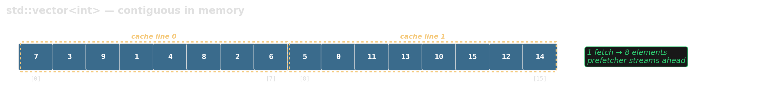
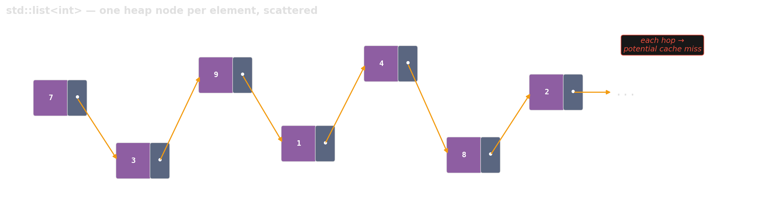
The choice decides the layout

Same sixteen integers, two containers — two very different shapes in memory.

What a pointer hop actually costs

Level	Latency	Ratio
L1 cache	~1 ns	1×
L2 cache	~4 ns	4×
L3 cache	~12 ns	12×
Main memory	~100 ns	100×

Order-of-magnitude numbers; exact values are hardware-specific.

A std::vector traversal lets the prefetcher keep data in cache.

A std::list traversal risks main memory on every hop.

Asymptotically identical, empirically one hundred times slower.

When does `std::list` actually win?

Three conditions, all at once:

Many splices, few traversals. Moving elements between lists without copying.
Iterator stability matters. Pointers into the list must survive insertions and removals elsewhere.
Elements are expensive to move. Copying or moving a value is costly compared to the pointer overhead.

If you cannot name all three, reach for std::vector.

`std::deque` — the Swiss army knife nobody should open

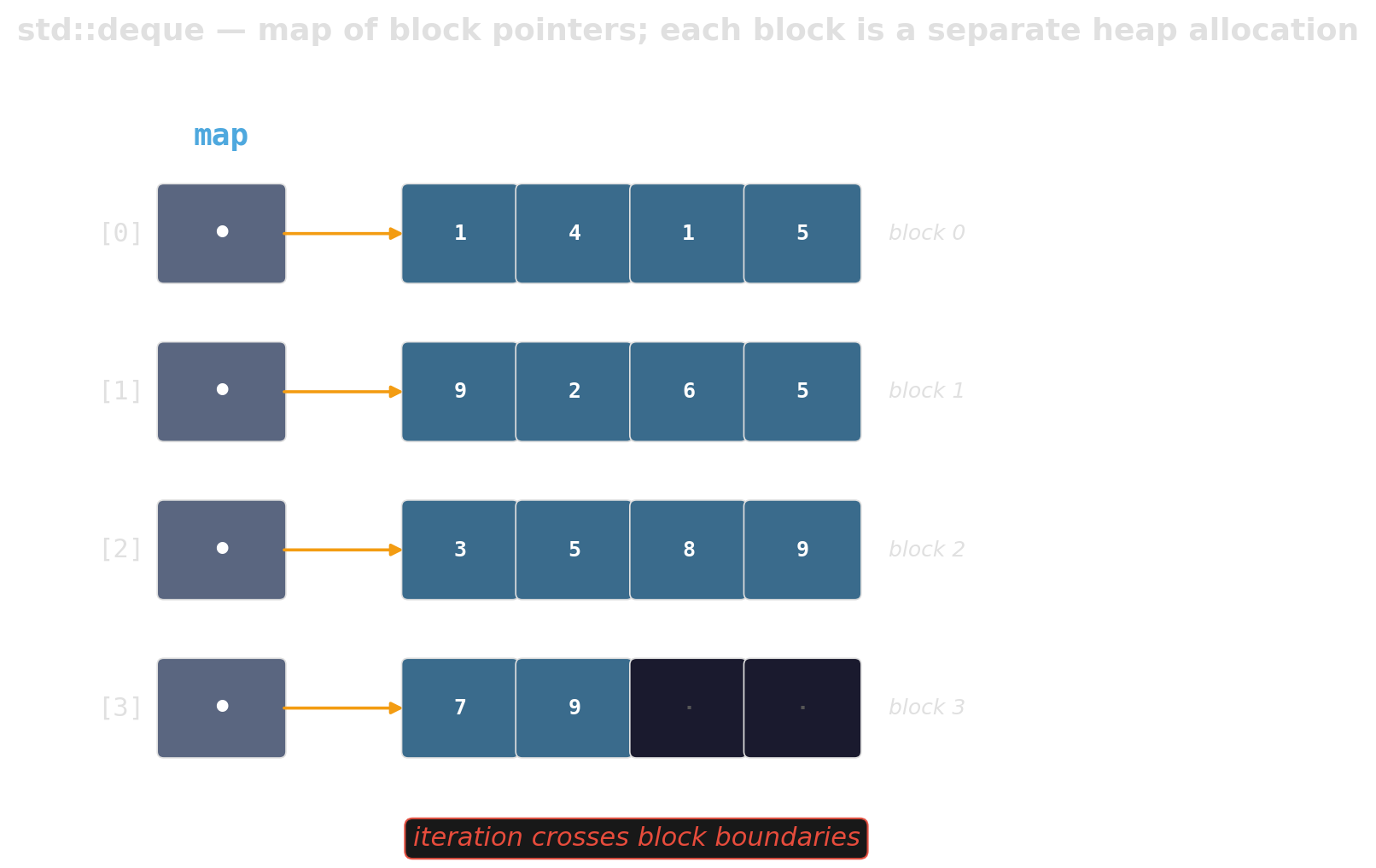
A map of pointers to blocks. Every iterator increment risks crossing a block boundary; every implementation is slightly different and usually slower than its specification suggests.

Prefer vector-as-queue

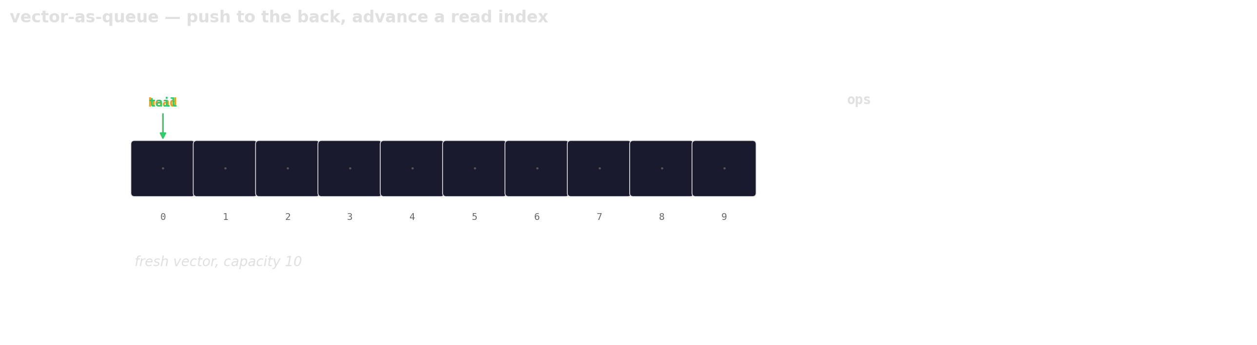
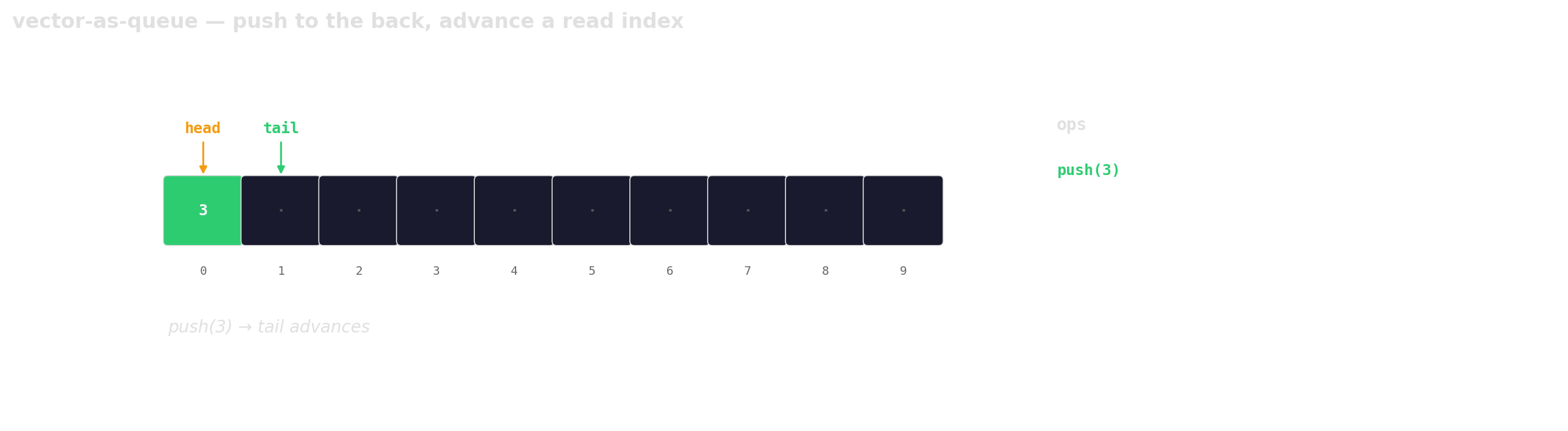
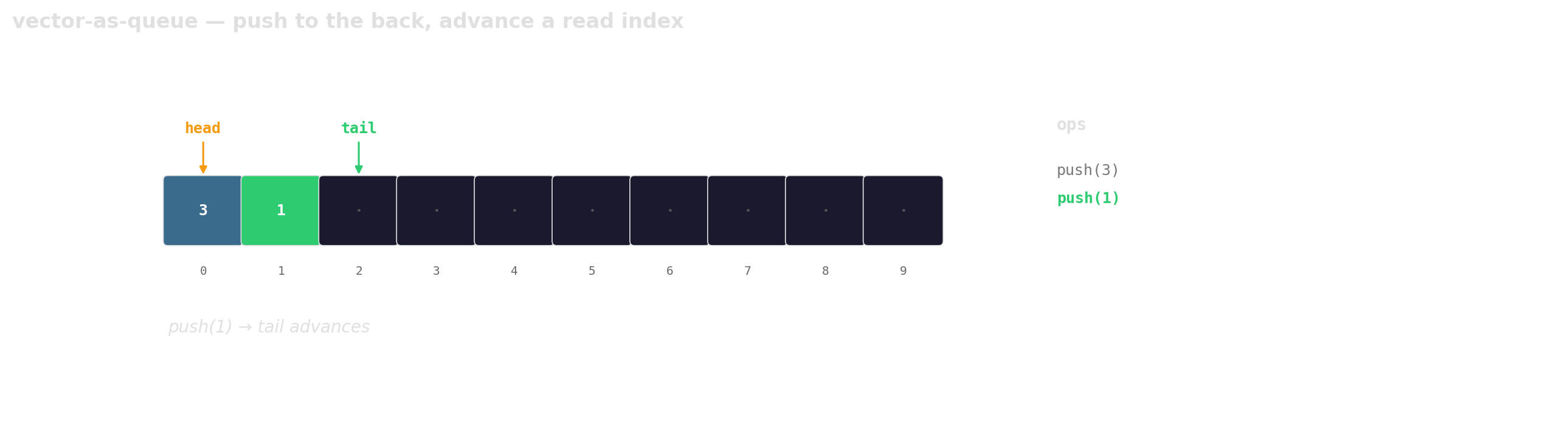
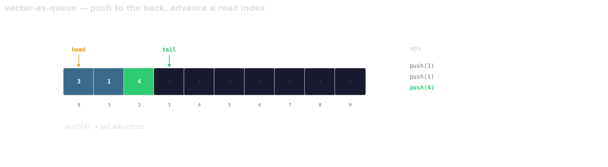
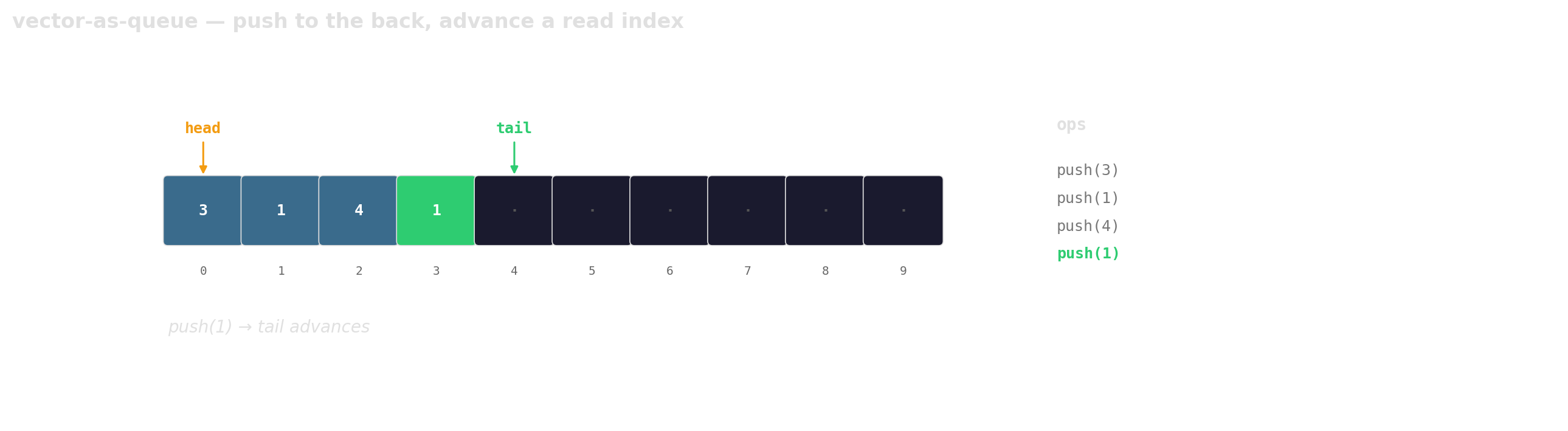
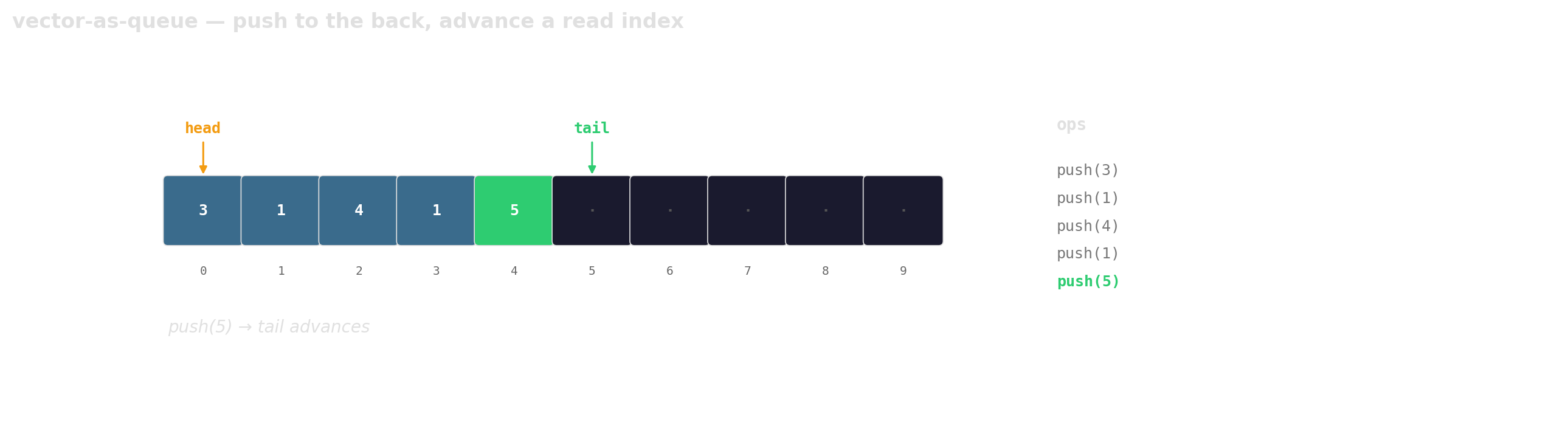
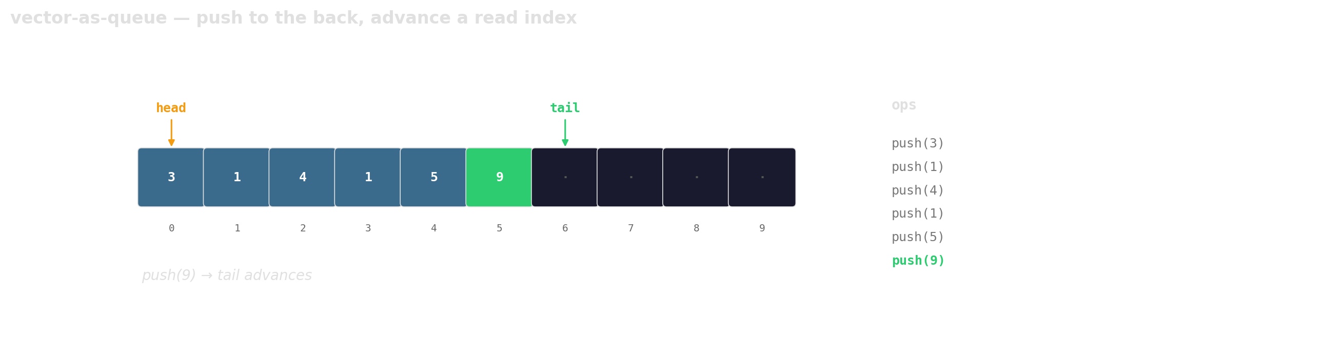
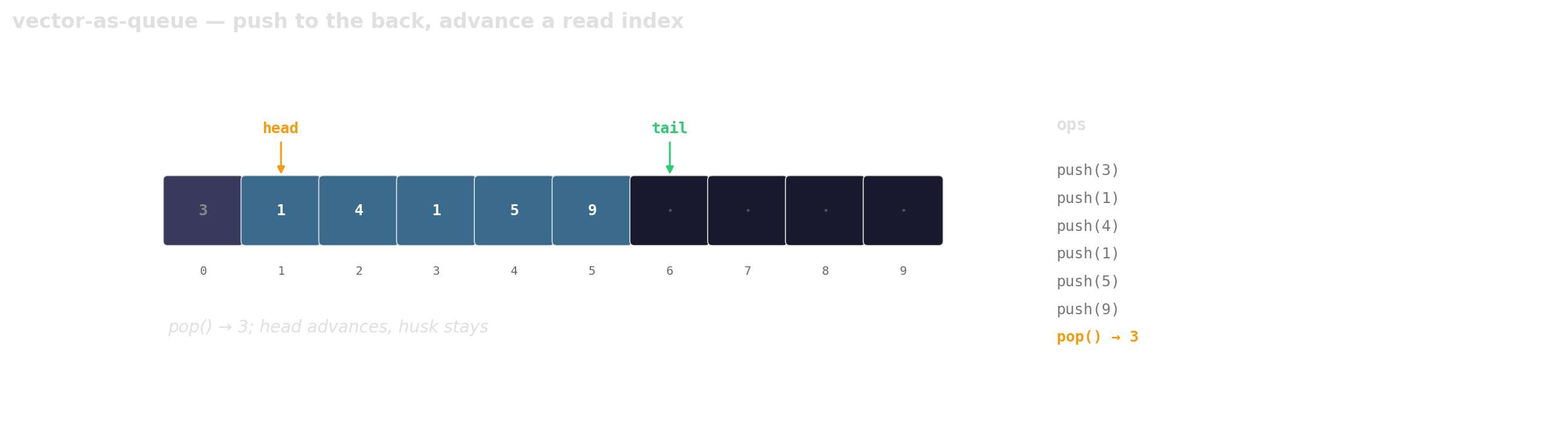
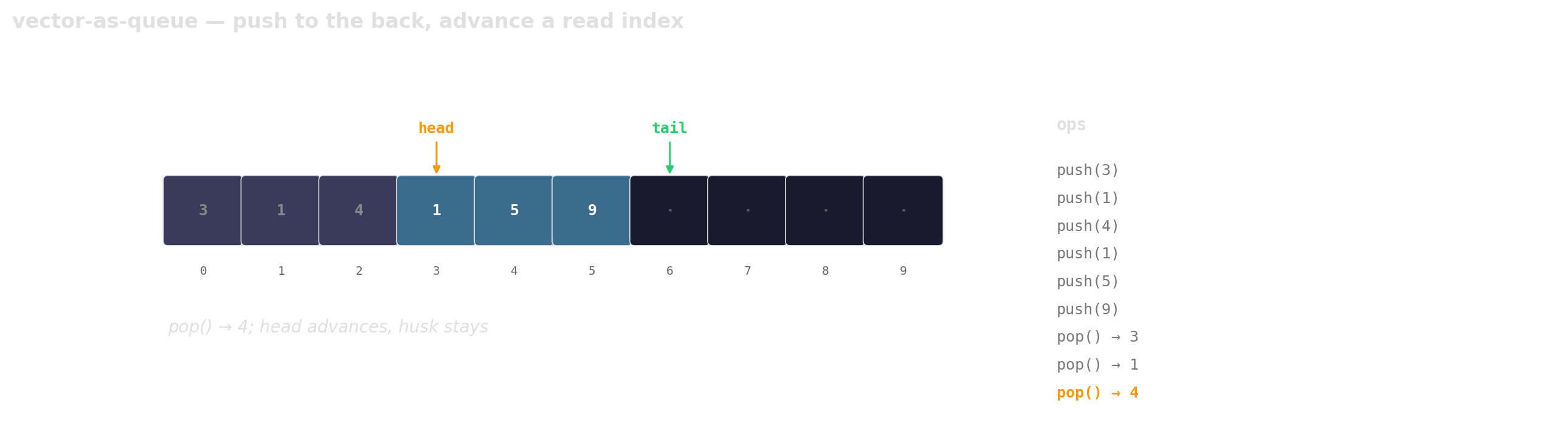
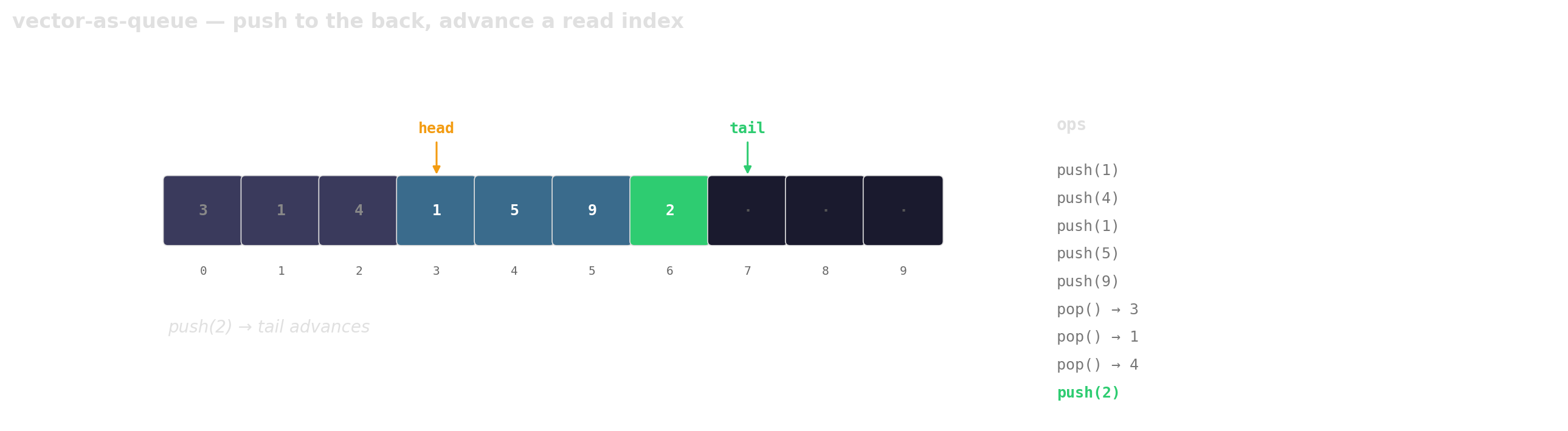
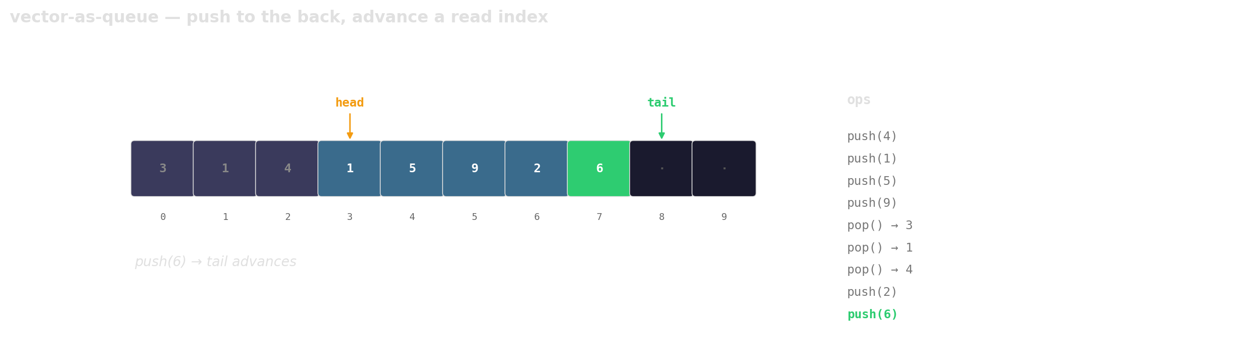
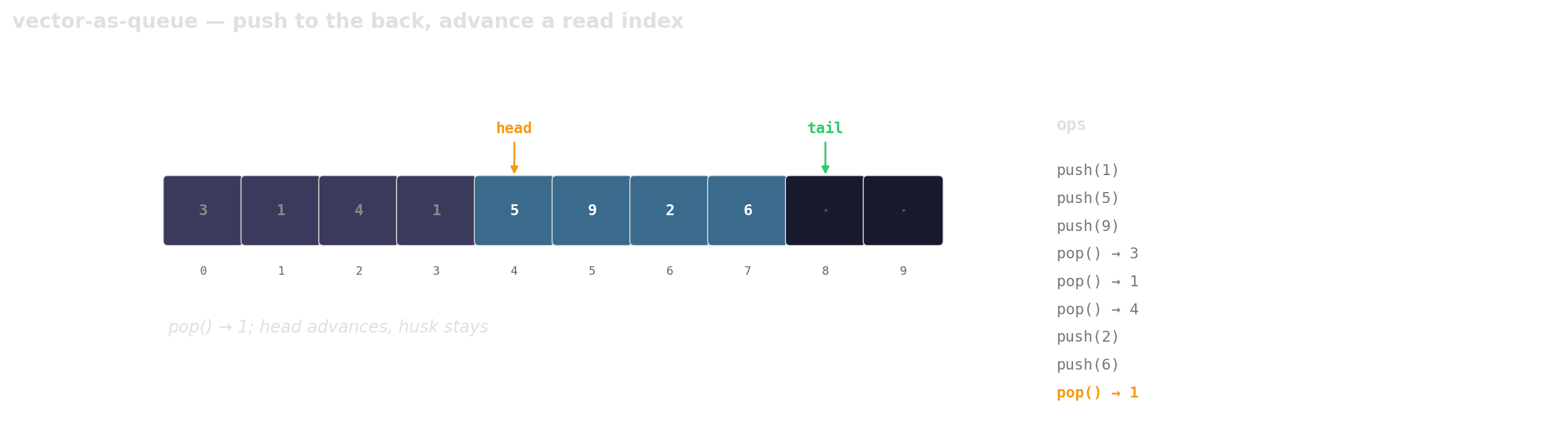
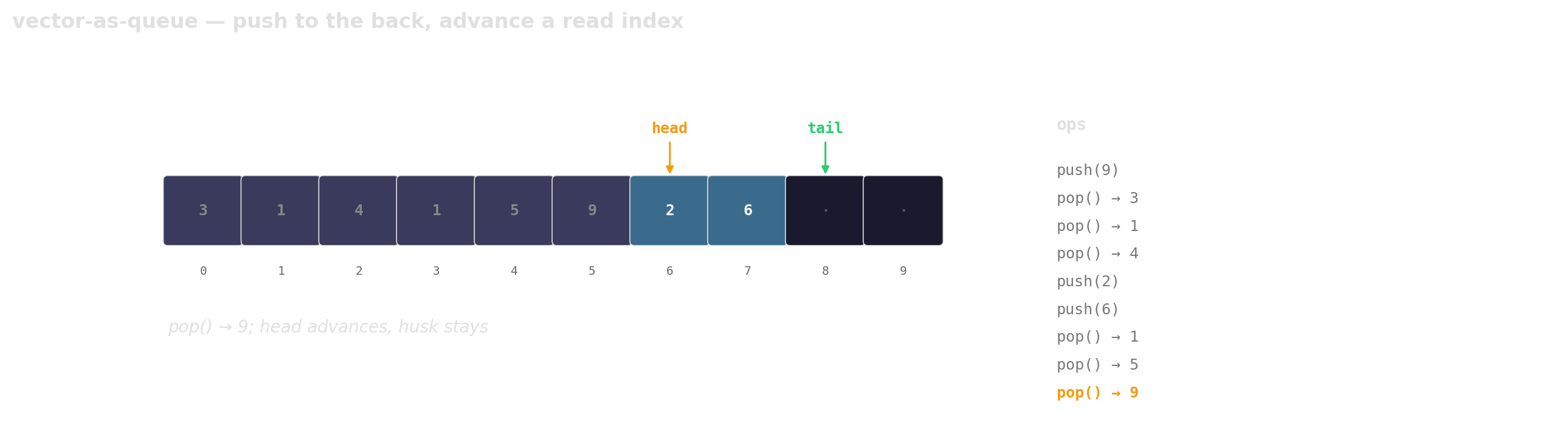
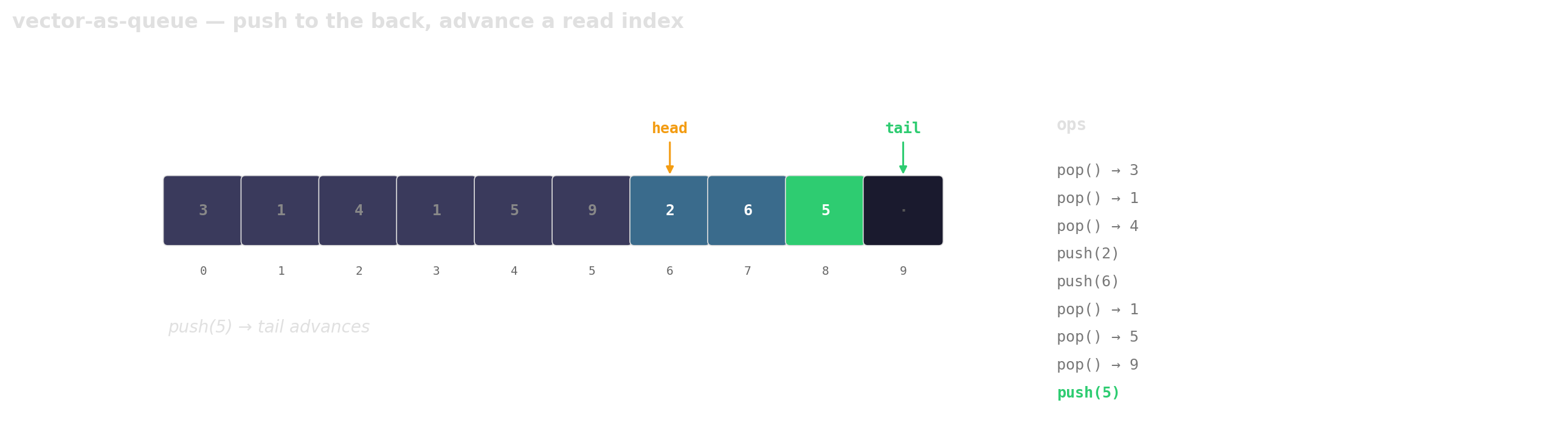
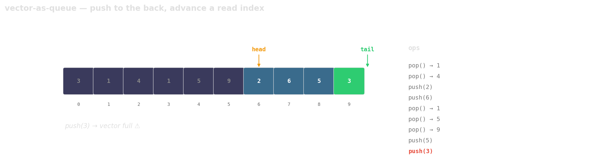
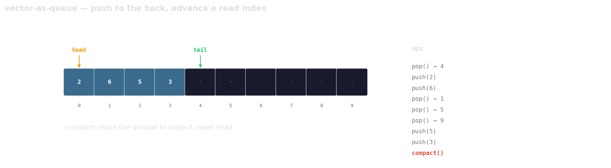
Trade a little memory (the husks) for contiguous layout, a single allocation, and one cache line per hop.

Small-buffer optimization

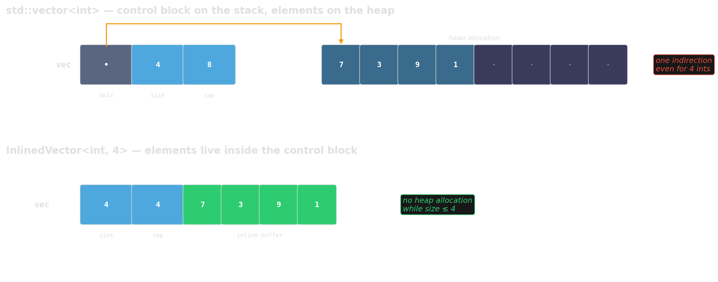
Worth reaching for: absl::InlinedVector, boost::small_vector, llvm::SmallVector.

Summary — linear structures

Default: std::vector. Contiguous, predictable, cache-friendly.
Last resort: std::list. Only when splicing, stable iterators, or expensive moves demand it.
Avoid: std::deque. Prefer std::vector with a read index.
Optimize small cases: absl::InlinedVector and friends when most instances hold only a handful of elements.

Carpenter, Almost Always Vector, CppCon 2024 (Carpenter 2024)
Carruth, High Performance Code 201: Hybrid Data Structures, CppCon 2016 (Carruth 2016)

Hash Maps

A core workhorse — with performance that depends heavily on the implementation.

When do we actually reach for a hash map?

Small N (≲ 100): sorted std::vector + linear scan — cache beats asymptotics.
Dense integer keys: std::vector<Value> indexed directly — no hash needed.
Ordered queries (range, predecessor): sorted container, not a hash map.
Everything else: hash map territory. But not the one the standard ships.

// Graph: map node_id (0..N-1) → degree.
std::vector<int> degree(N, 0);
for (auto e : edges) degree[e.src]++;

// Tokenized text: count by token ID.
std::vector<int> count(vocab_size, 0);
for (auto tok : tokens) count[tok]++;

`std::unordered_map` is a linked list in disguise

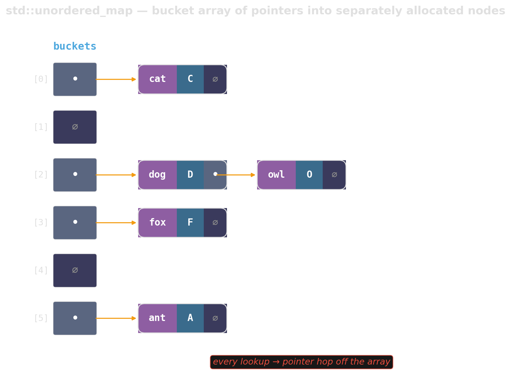
The bucket array holds pointers to heap-allocated nodes. Every insert allocates; every lookup chases a pointer off the array.

Open addressing — keep collisions local

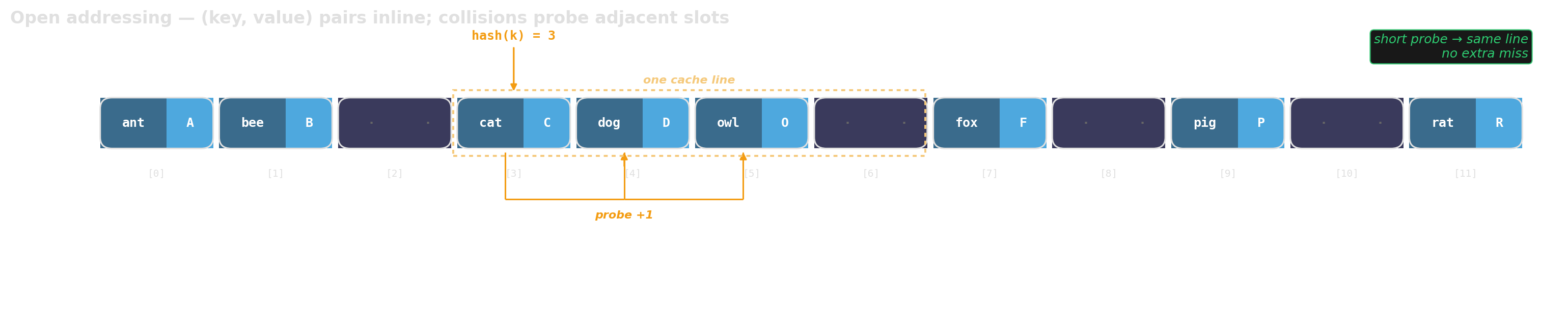
One allocation. Collisions probed in adjacent slots. A miss stays in the same cache line.

But: wide values → few slots per cache line. Every probe step = fresh cache line.

Swiss tables — split metadata from data

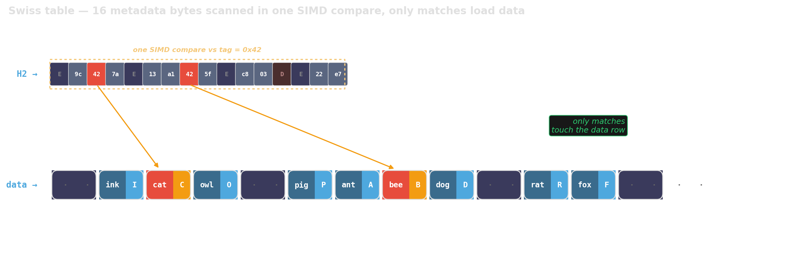
Tiny metadata array scanned before any key is touched — 16 slots per cache line, regardless of value width.

A single SIMD instruction checks all 16 tags at once; only matches pay to read the full key-value pair.

Tuning: reserve, load factor, hash quality

Reserve before a bulk insert — one call avoids ~log of N rehashes.
Load factor: leave it alone. The defaults are benchmarked.
Hash quality: std::hash<int> is typically the identity. Swap in xxHash or ankerl::unordered_dense::hash for hot string keys.

Summary — hash maps

Check the exceptions first: dense integer keys → std::vector. Ordered queries → sorted container. Tiny N → linear scan.
Avoid: std::unordered_map. Chained by standard mandate — 2× slower on hits, 3–4× on misses and unreserved build.
Default: ankerl::unordered_dense, absl::flat_hash_map, or boost::unordered_flat_map.
Tune: reserve before bulk inserts. Leave load factor alone. Hash quality matters for non-trivial keys.

Sorted Containers

When order itself is part of the query, not just membership.

When do we actually need order?

Range queries: “all log entries between 10:00 and 11:00”, “prices between 90 € and 110 €”
Predecessor / successor: “closest timestamp ≤ now”, “next larger key”
Ordered iteration: stream keys sorted, merge two indexes, prefix scans
Order statistics: k-th smallest, rank of a key
Database / filesystem indexes: every B-tree on disk exists for range scans

If none of these apply, you want a hash map, not a sorted container.

Lead with the simplest thing: sorted `std::vector`

Build once, binary-search many times.

std::vector<std::pair<Key, Value>> table;
// ... fill and sort by key ...

auto it = std::lower_bound(
    table.begin(), table.end(), key,
    [](auto const& p, Key const& k) { return p.first < k; });

if (it != table.end() && it->first == key) {
    use(it->second);
}

Read-mostly ordered map? Start here. Simple and fast.

`std::map` is a red-black tree

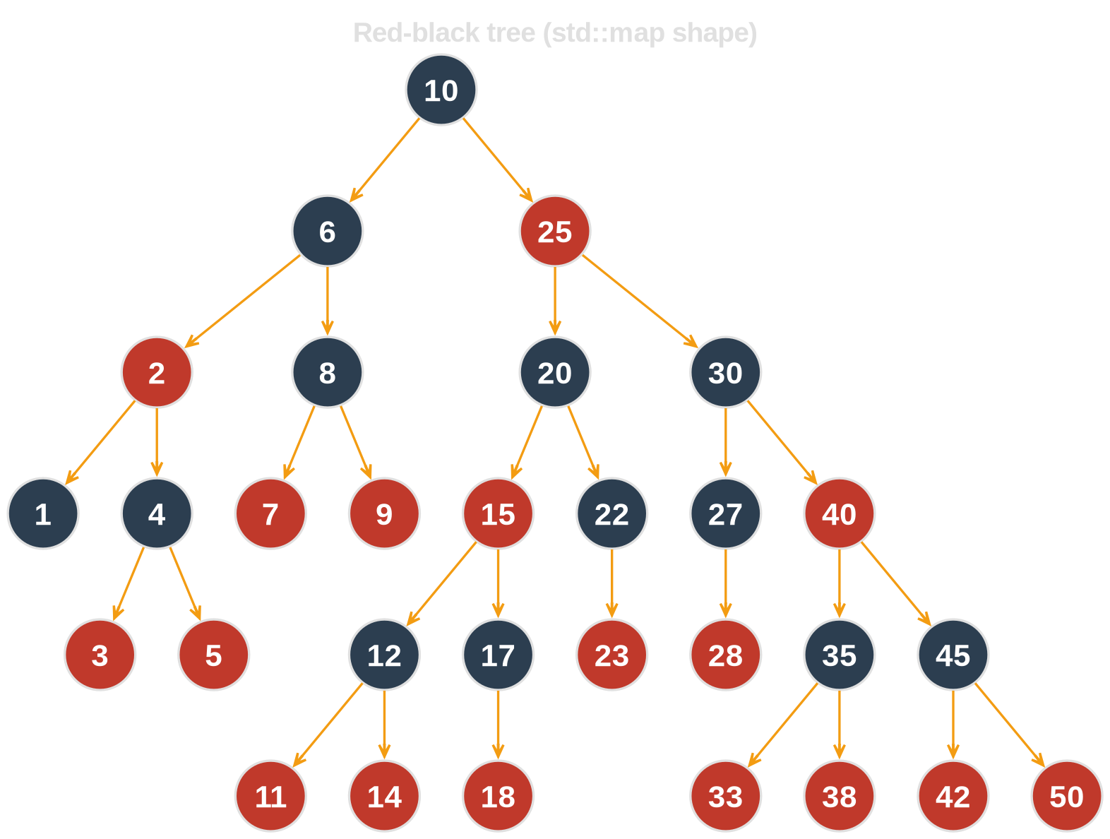
30 keys → 30 separate allocations, 6 levels deep. std::map is std::list with a sorting invariant — per-node malloc, plus rebalancing on every insert.

Height is the cost

For one million keys, a balanced binary tree is ~20 levels deep.

Each level is a pointer hop to somewhere else in memory. In the bad case, 20 cache misses per lookup — and the work inside each node is negligible.

Cache misses come from tree height, not from node work. Reduce height by widening the branching factor.

B-tree: same keys, one cache line per node

30 keys → 13 nodes, 3 levels (order 5). Every key still carries its own value pointer (gray stubs).

Node sized to one cache line ⇒ one cache miss per level ⇒ logarithm in the branching factor, not in two.

Choosing the order: match the cache line

In memory: order 16–64. Node fits in one or two cache lines.
On disk: order 128–512. Node is a disk block; minimize seeks.
Bigger nodes ⇒ more work inside the node, diminishing returns on height.

Same structure, different constant. The “latency you are minimizing” decides the node size.

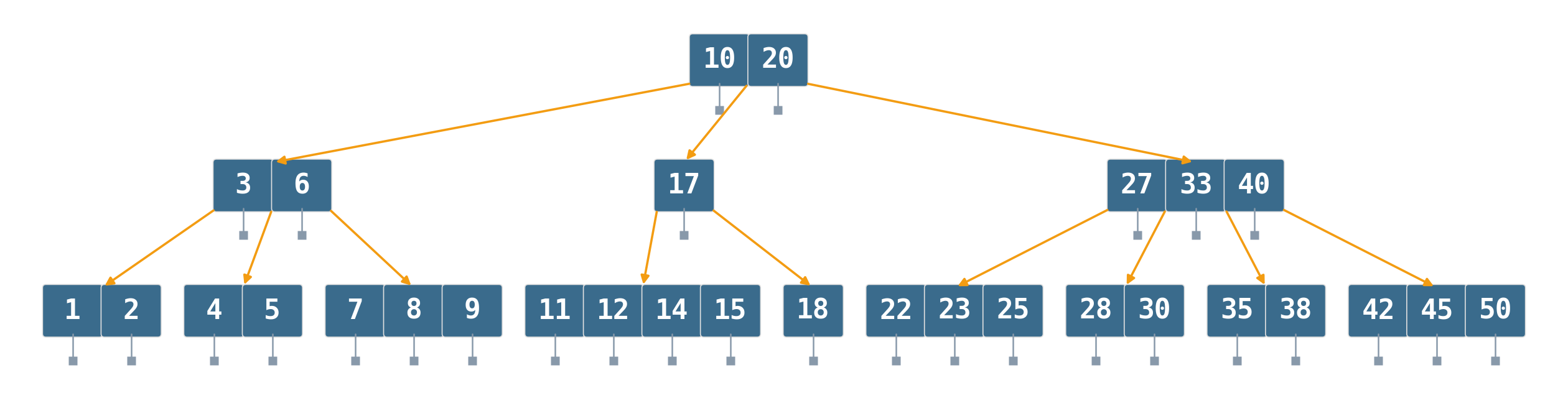
B+ tree: routing on top, values in leaves

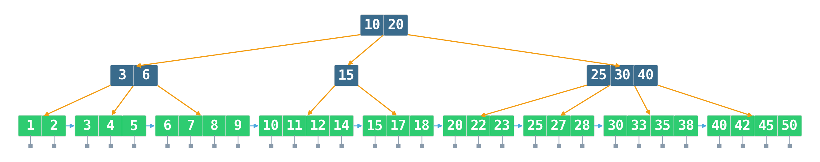
Internal nodes = pure routing. All values live in leaves. Leaves linked for range scans.

Range query = one tree descent + a linear walk over the leaf chain. This is why every database uses B+.

Summary — sorted containers

Ask first: do I need order, or just point lookup? If lookup only → hash map.
Default: sorted std::vector + lower_bound. Build once, search many — but mid-insert is O(N): on a million-key vector a single insert shifts megabytes.
Mutation-heavy ordered map: absl::btree_map. Drop-in for std::map, ~3× faster lookup, per-op cost stays bounded by log N.
Range scans dominate: B+ tree or sorted vector — sequential memory layout, no pointer-chasing.
Avoid: std::map. Red-black tree with per-node malloc — slower than absl::btree_map on every workload. No shape where it wins.

Priority Queues

The simple binary heap is the right default — with one useful tuning knob.

When do we actually need a priority queue?

Event simulation: “what happens next?” ordered by time stamp
Shortest paths / A*: expand the frontier vertex with the smallest tentative distance
Top-k selection: keep a bounded heap of the best k items in a stream
Scheduling: earliest-deadline-first, anytime-algorithm re-queues
Branch-and-bound: always explore the cheapest open node first

If you only need the ordering once at the end, just sort. A priority queue earns its place when you pop and keep inserting.

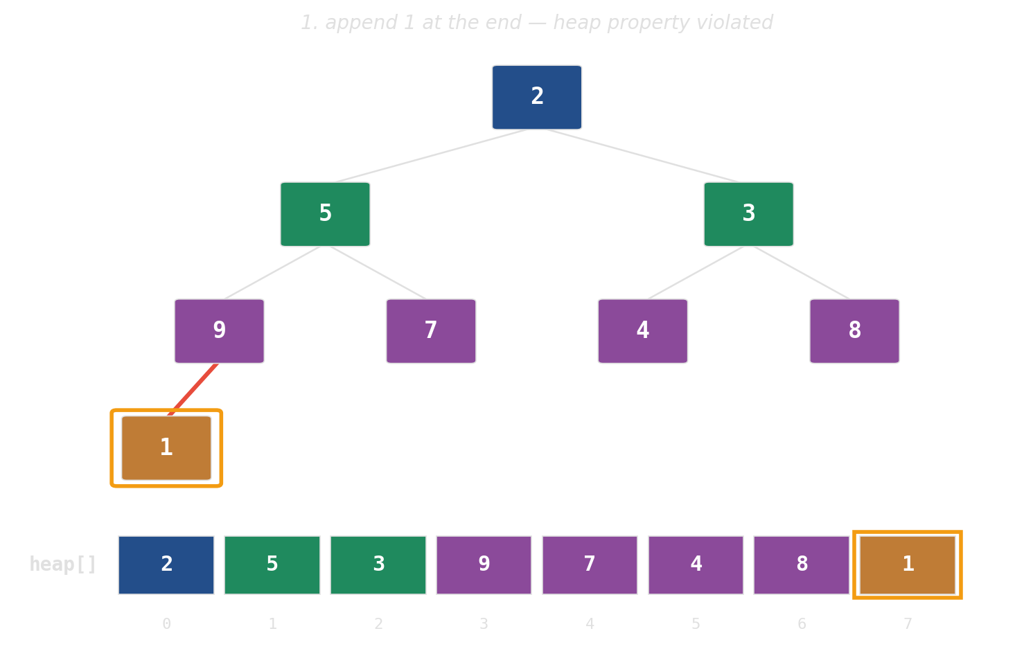
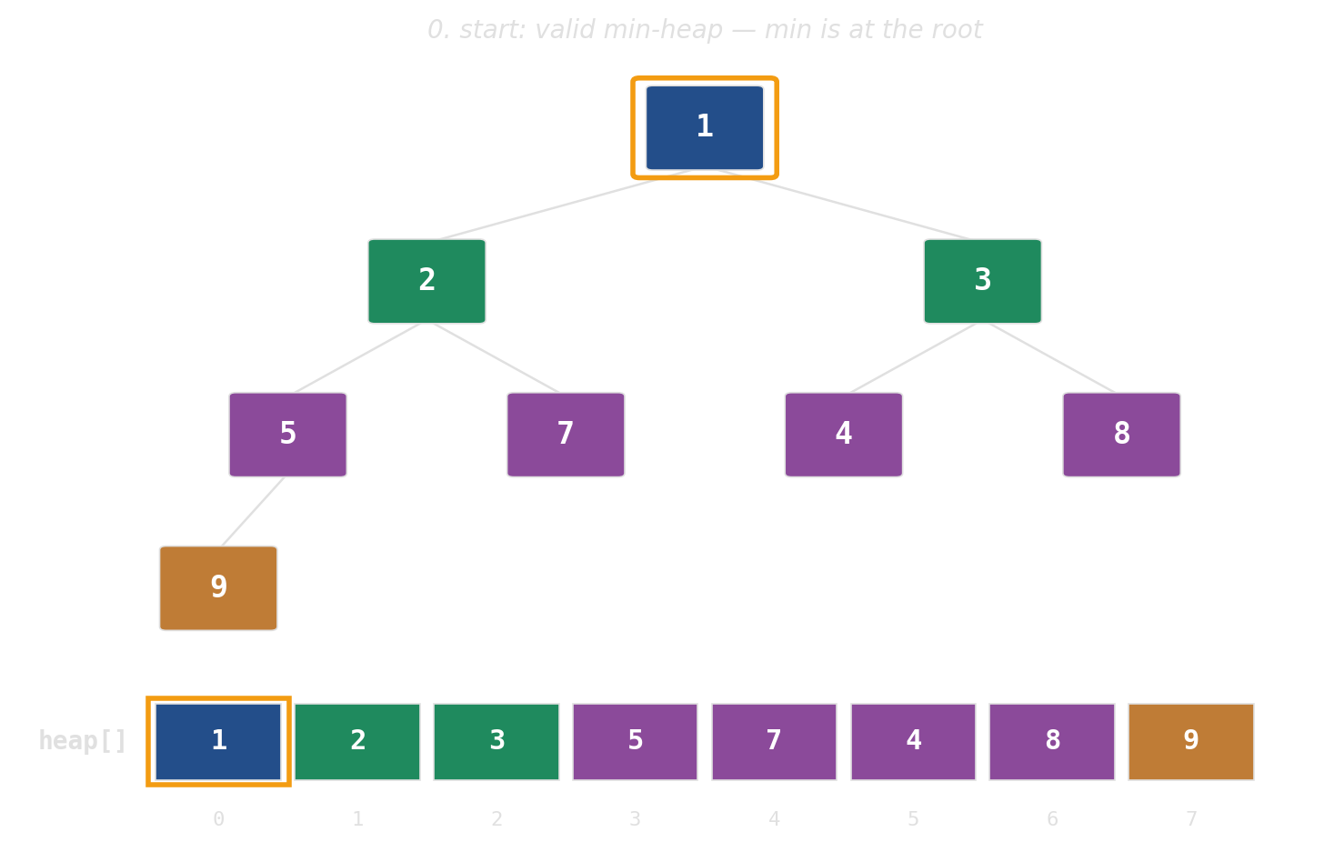
Binary heap: implicit tree in a flat array

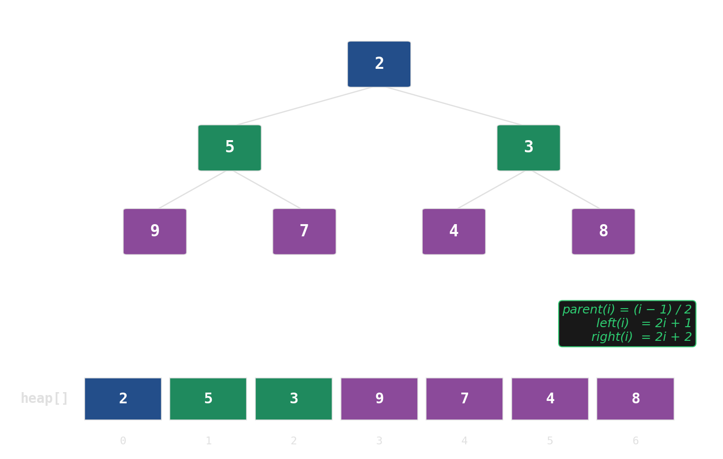
No pointers, no per-node allocations. The tree is index arithmetic on a std::vector.

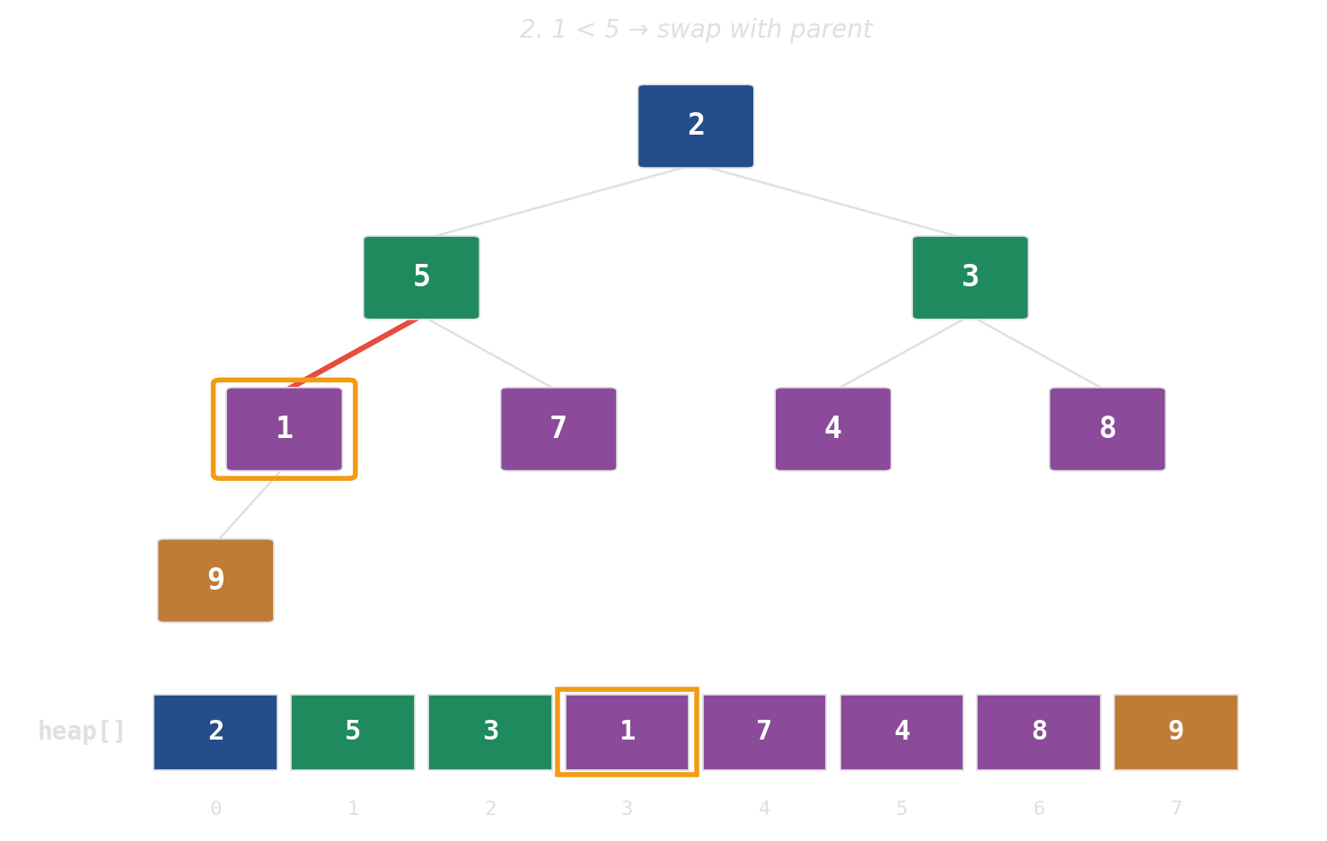
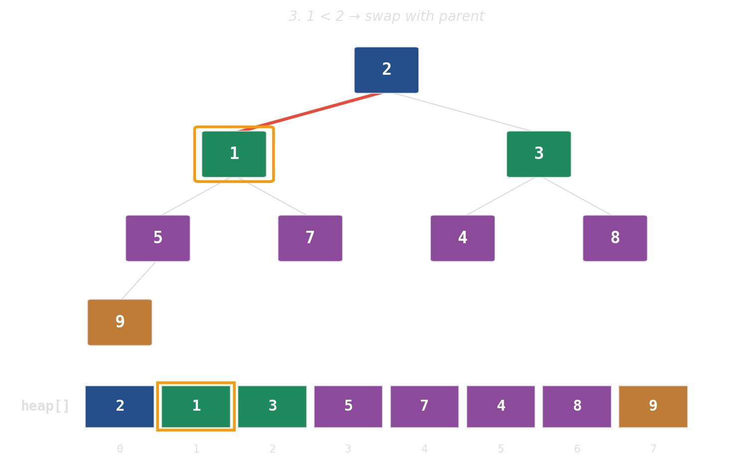
push: append, then bubble up

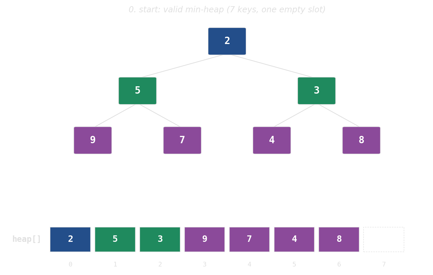
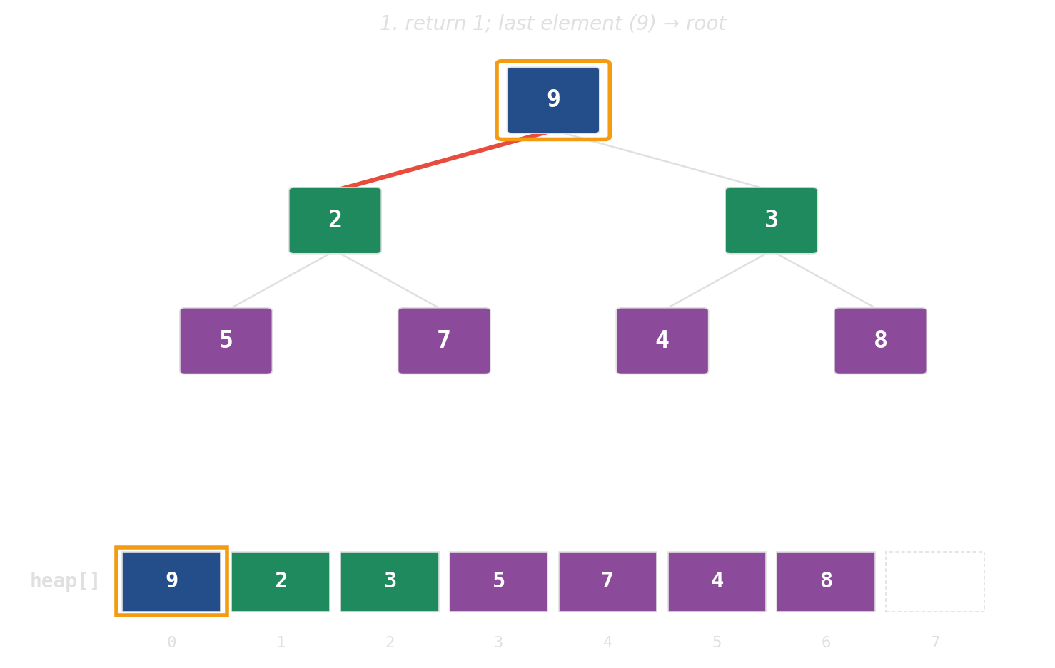
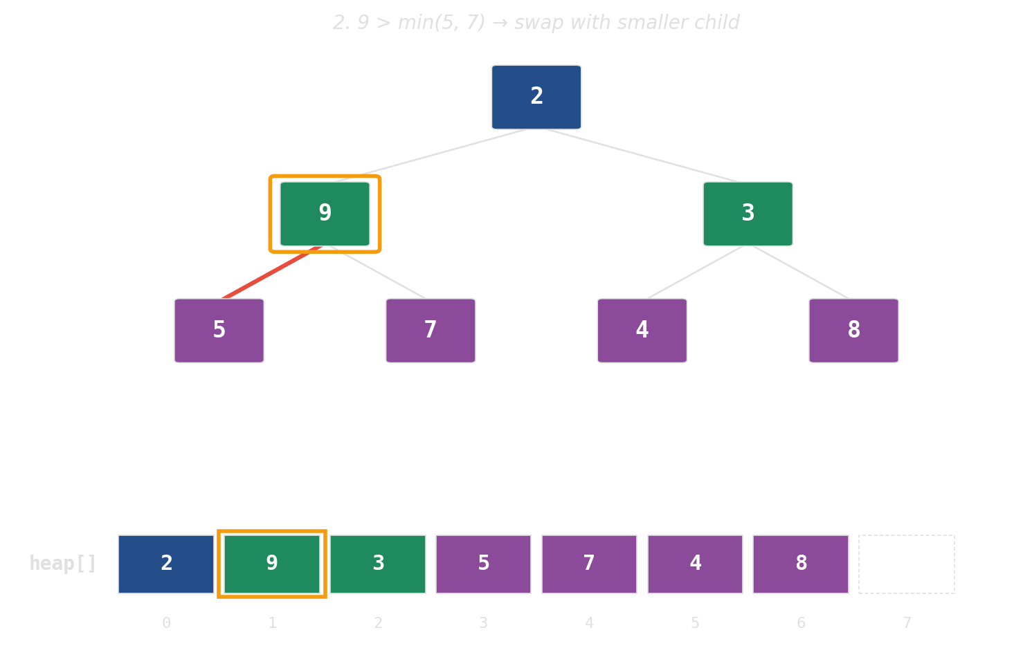
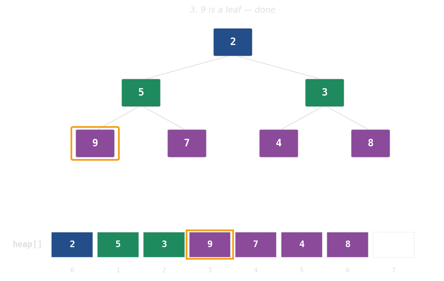
pop: swap root with last, then sift down

Height is the cost — widen the tree

A binary heap over one million keys is ~20 levels deep. Each level is a potential cache miss per push / pop. Widen the tree, shrink the height.

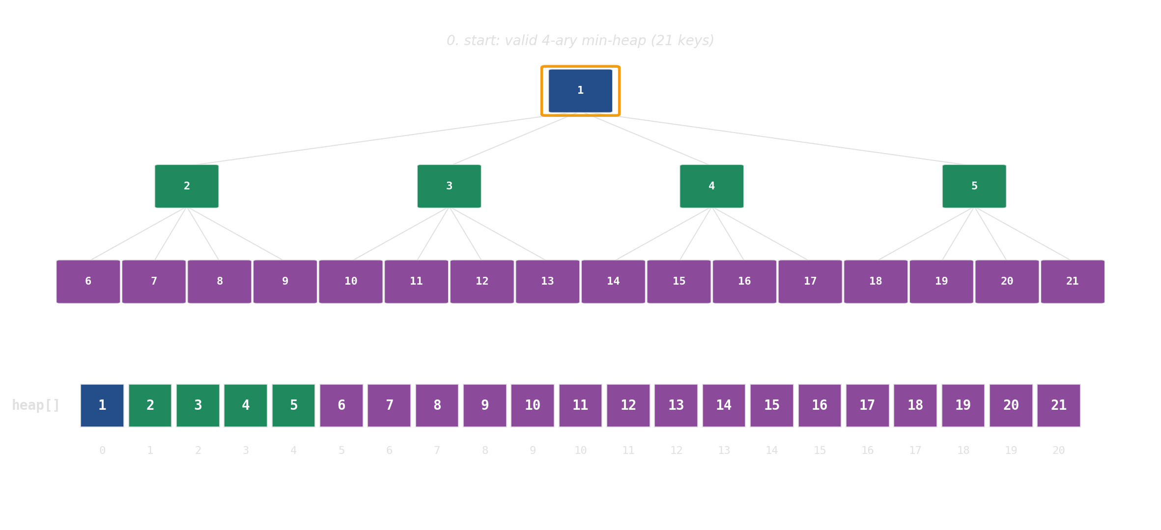
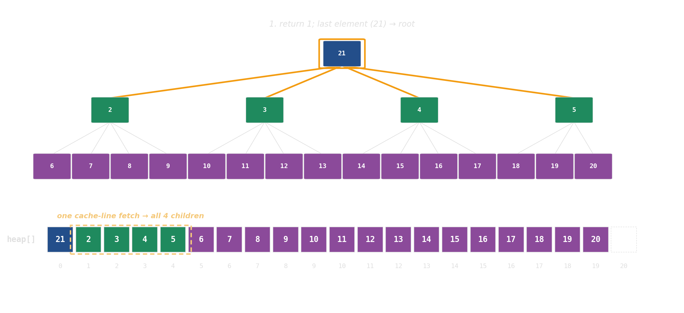
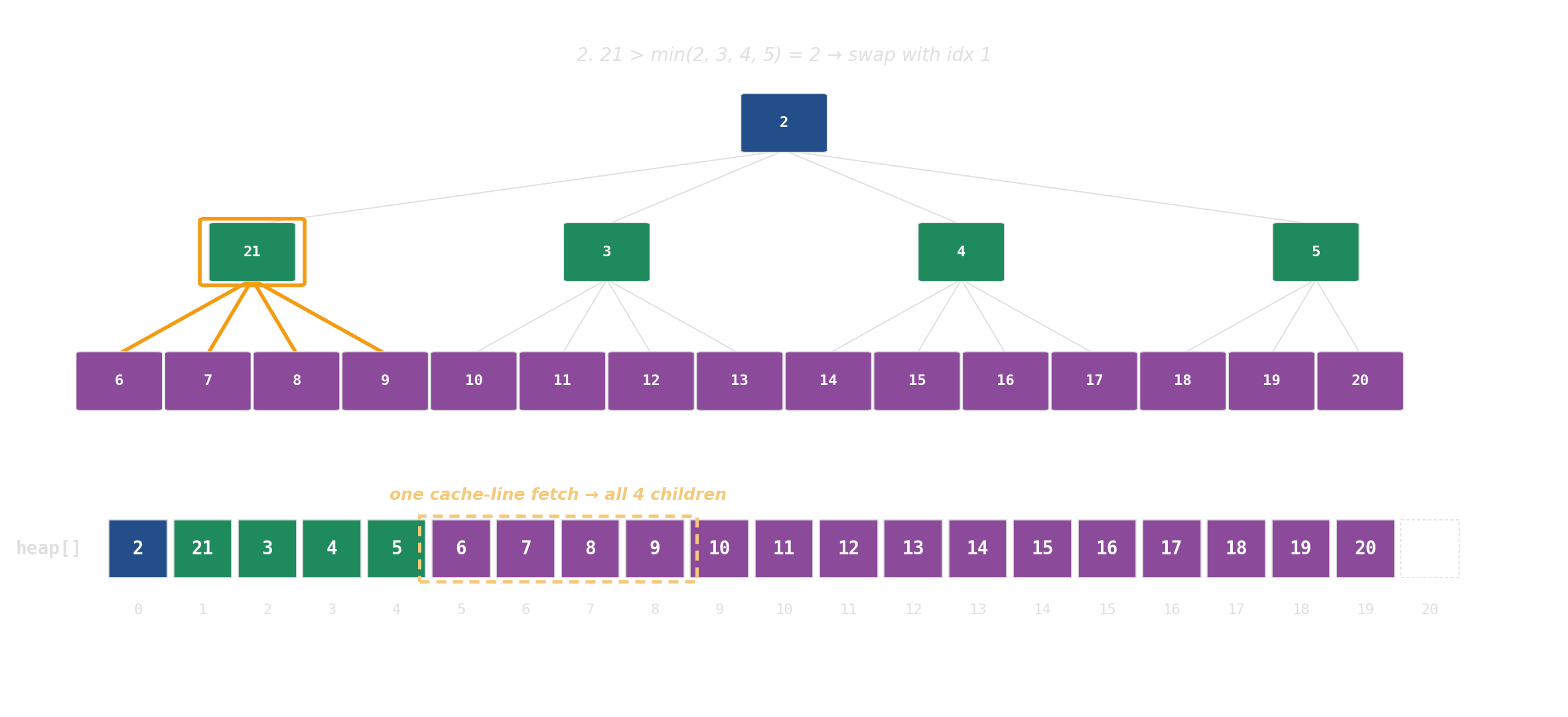
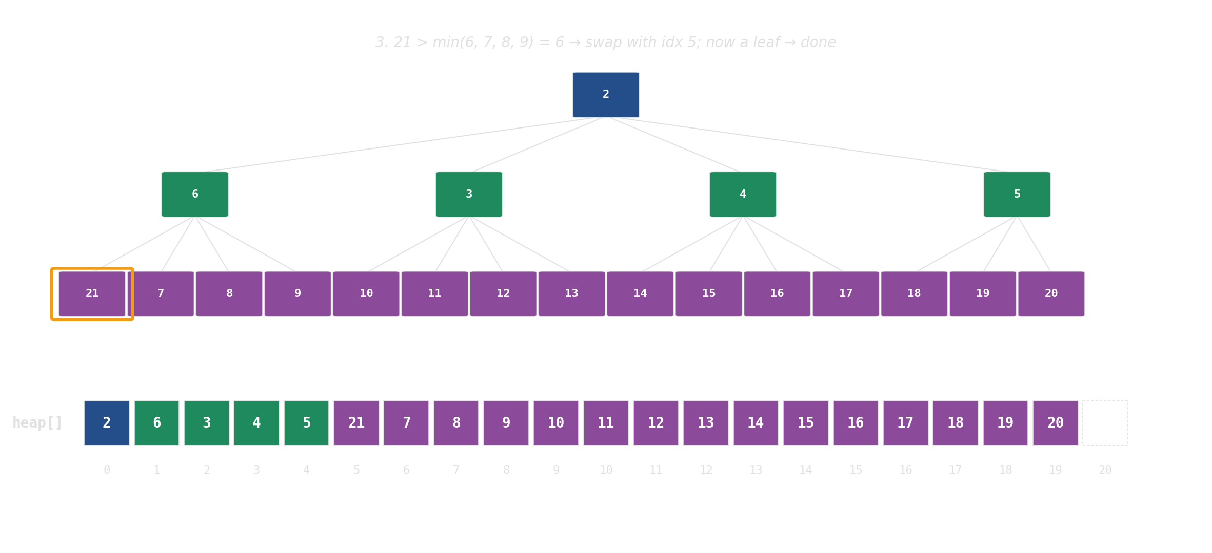
d-ary heap: each node has d children instead of 2. Same array, same index arithmetic — just d·i + k instead of 2i + 1. The d children sit in one cache line; height drops from log₂ N to log_d N.

Modifying the key? Push a new entry instead

Heaps support no efficient way to change a key already in the heap. Work around it:

// min-heap: smallest priority first
using Entry = std::pair<int, int>;           // (priority, id)
std::priority_queue<Entry, std::vector<Entry>, std::greater<>> pq;

pq.push({new_priority, id});                 // duplicate, not update

while (!pq.empty()) {
    auto [p, id] = pq.top(); pq.pop();
    if (p != priority[id]) continue;         // stale — skip
    process(id);
}

Lazy deletion. The heap grows by at most a constant factor per update — a cheap price for avoiding the reverse-index bookkeeping a real decrease-key needs.

Summary — priority queues

Ask first: push-and-pop in a loop? If it is “sort once at the end” → just std::sort.
Default: std::priority_queue — binary heap on a vector. Cache-friendly, no allocations.
Cheap knob: a d-ary heap (d = 4 or 8) if the heap is large.
Modifying a key? Lazy deletion.

Asymptotic ≠ fast — the Fibonacci heap. Better textbook bound for Dijkstra, but pointer-chasing and cache-hostile consolidation make it lose to a flat binary heap in practice. Lazy deletion removes the last reason to use it.

Union-Find

A case where the theory translates well into practice: a compact implementation with very low amortized cost.

Two operations

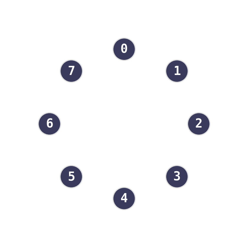
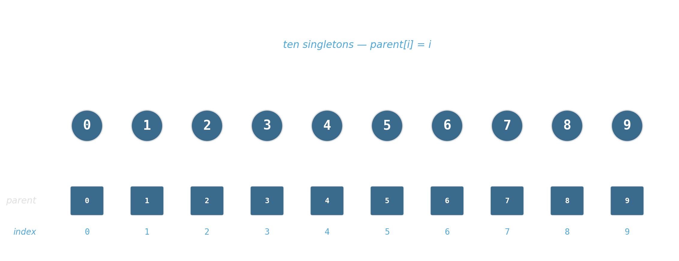
Maintain a partition of {0, …, 7} under:

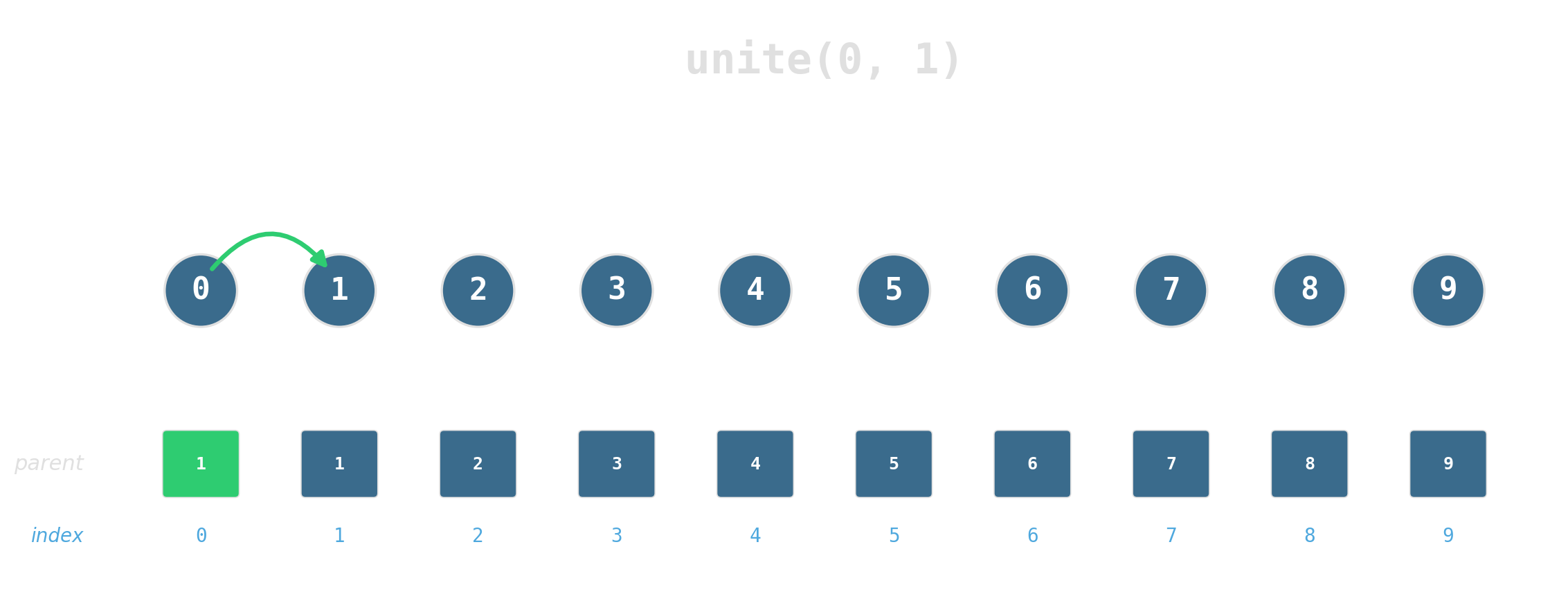
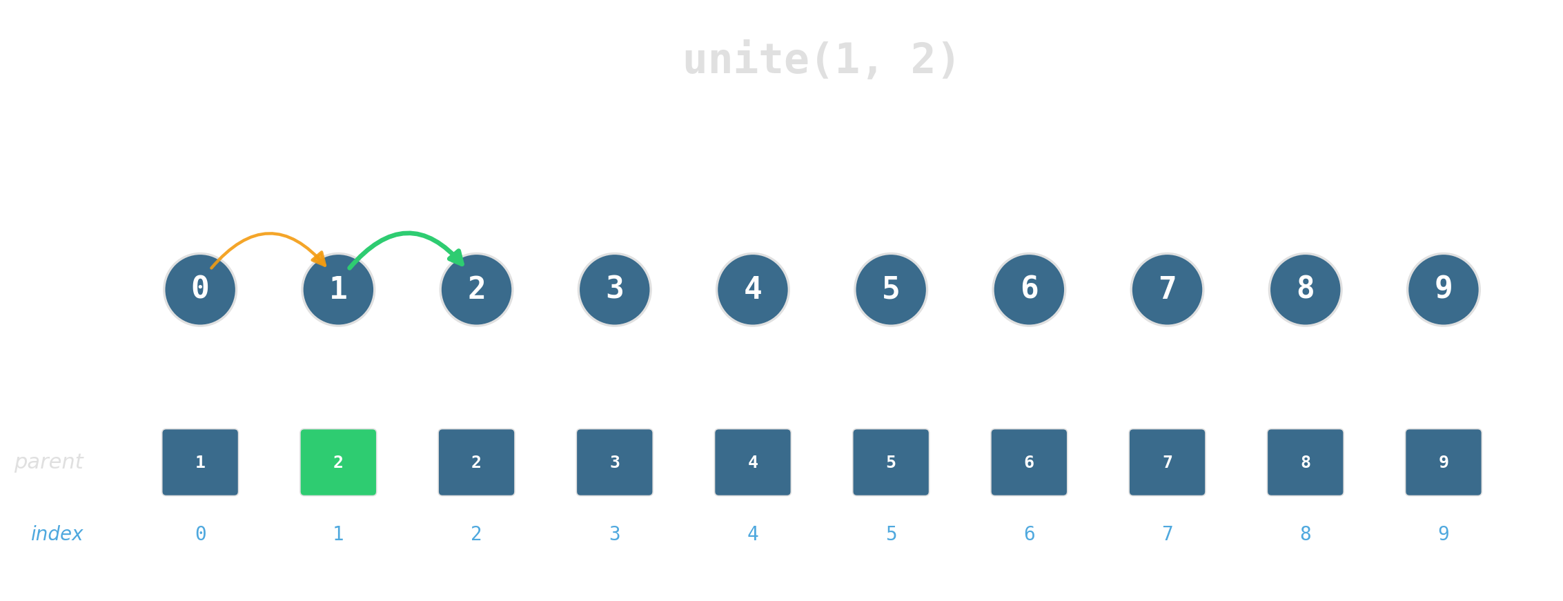
find(x) — which set is x in?
unite(x, y) — merge the two sets.

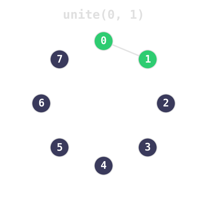
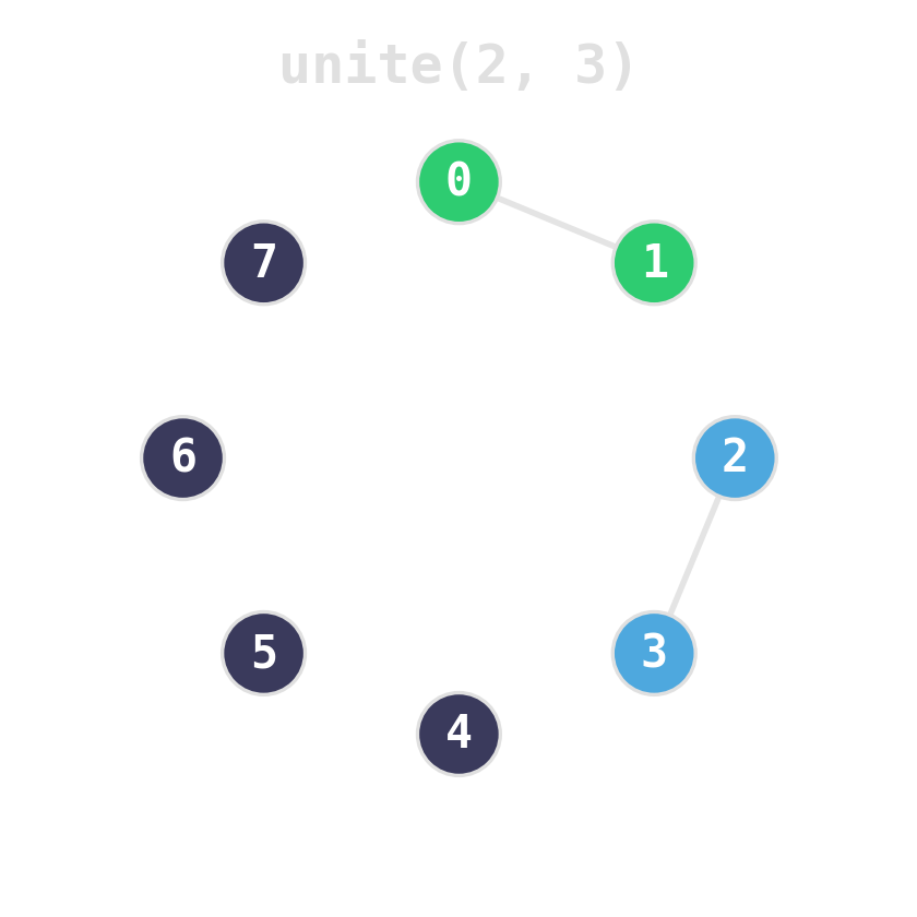
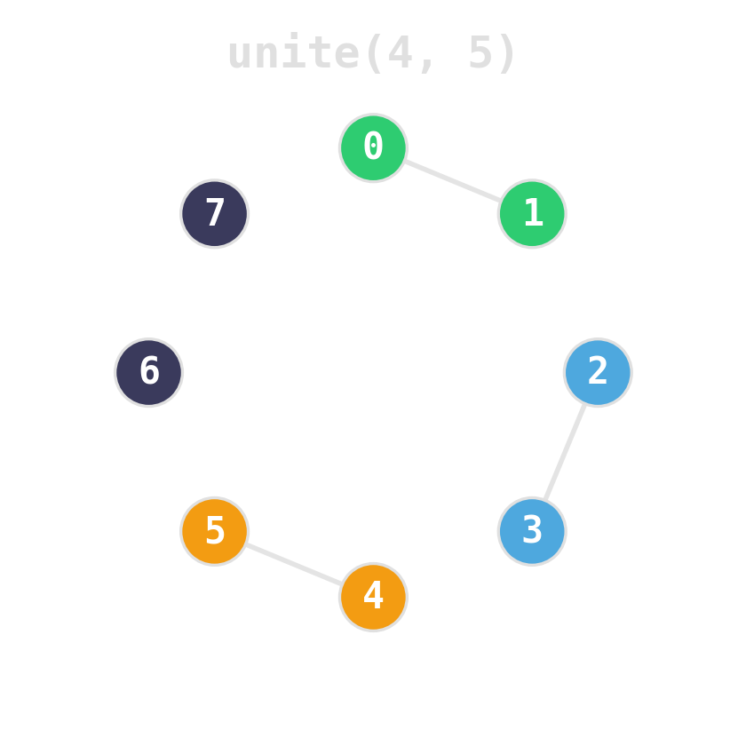
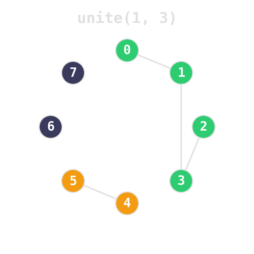
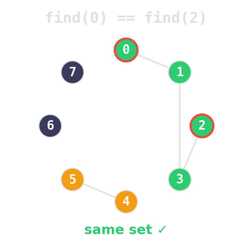
Two ideas, near-constant time

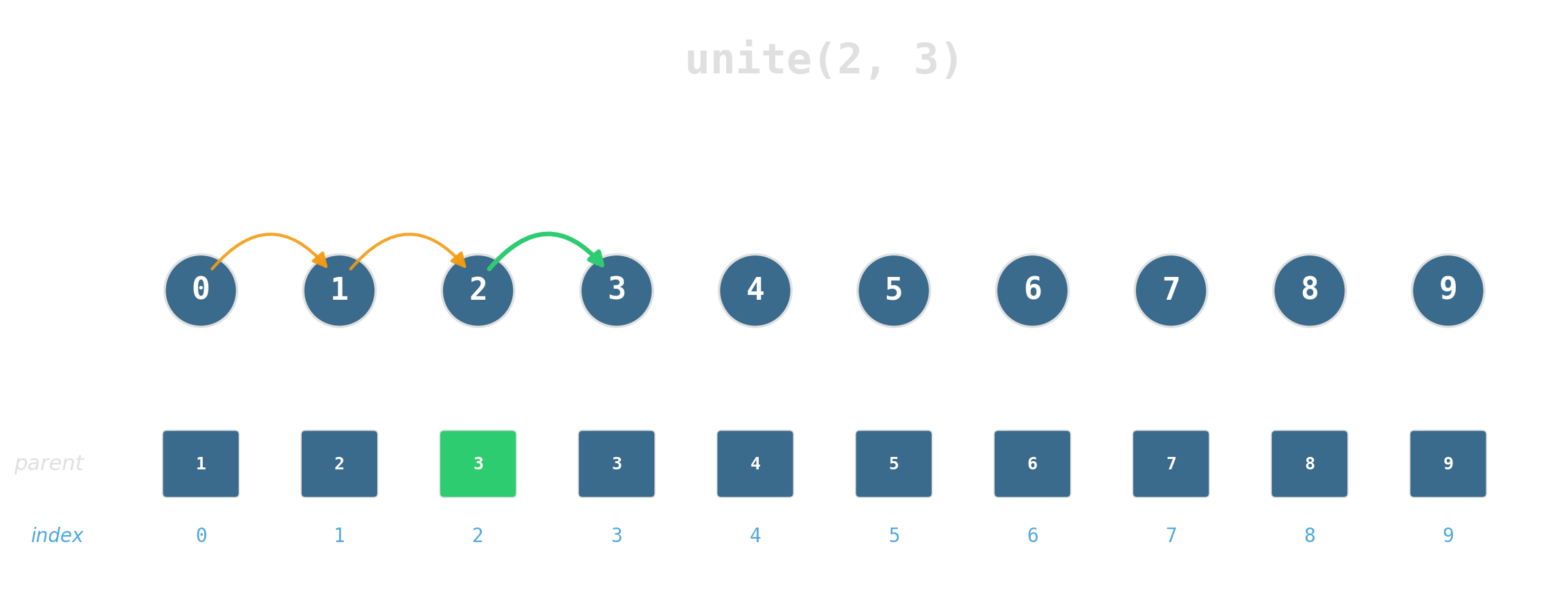
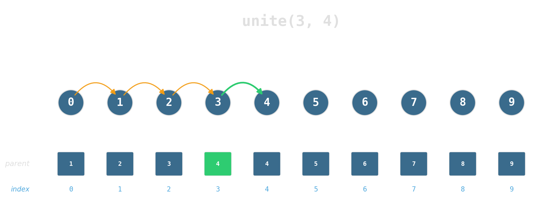
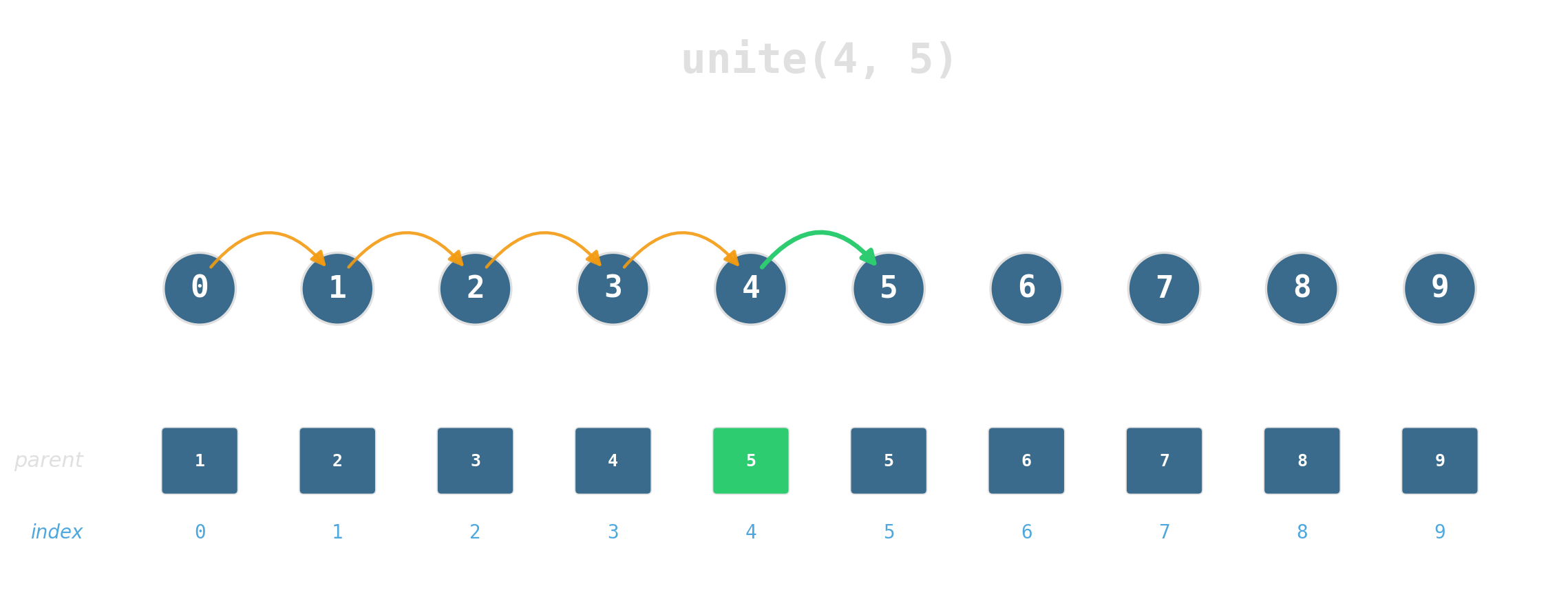
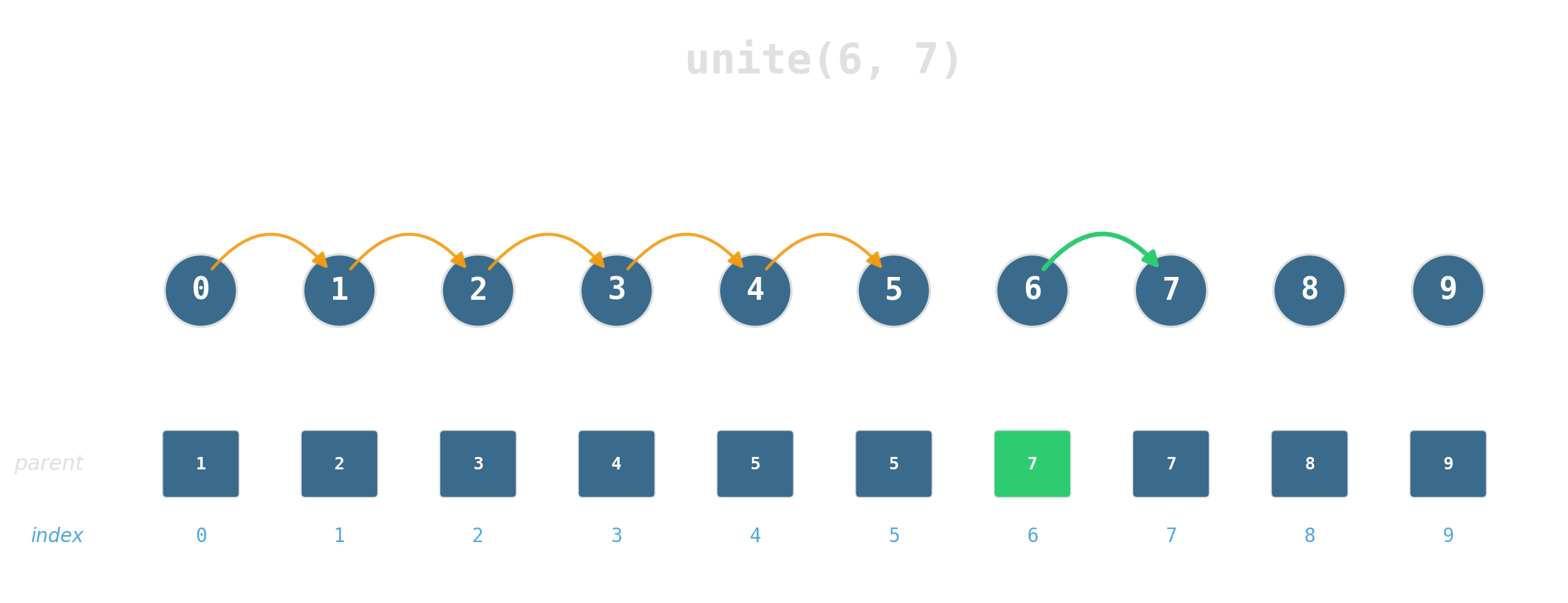
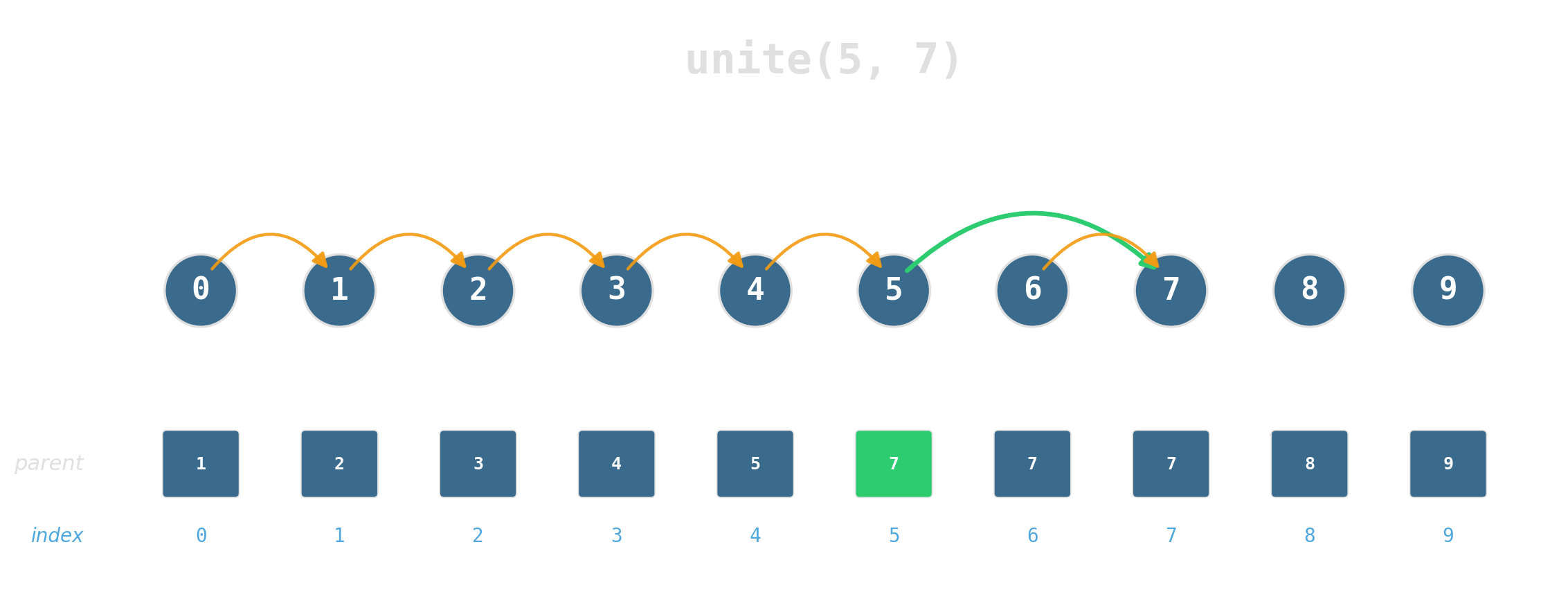
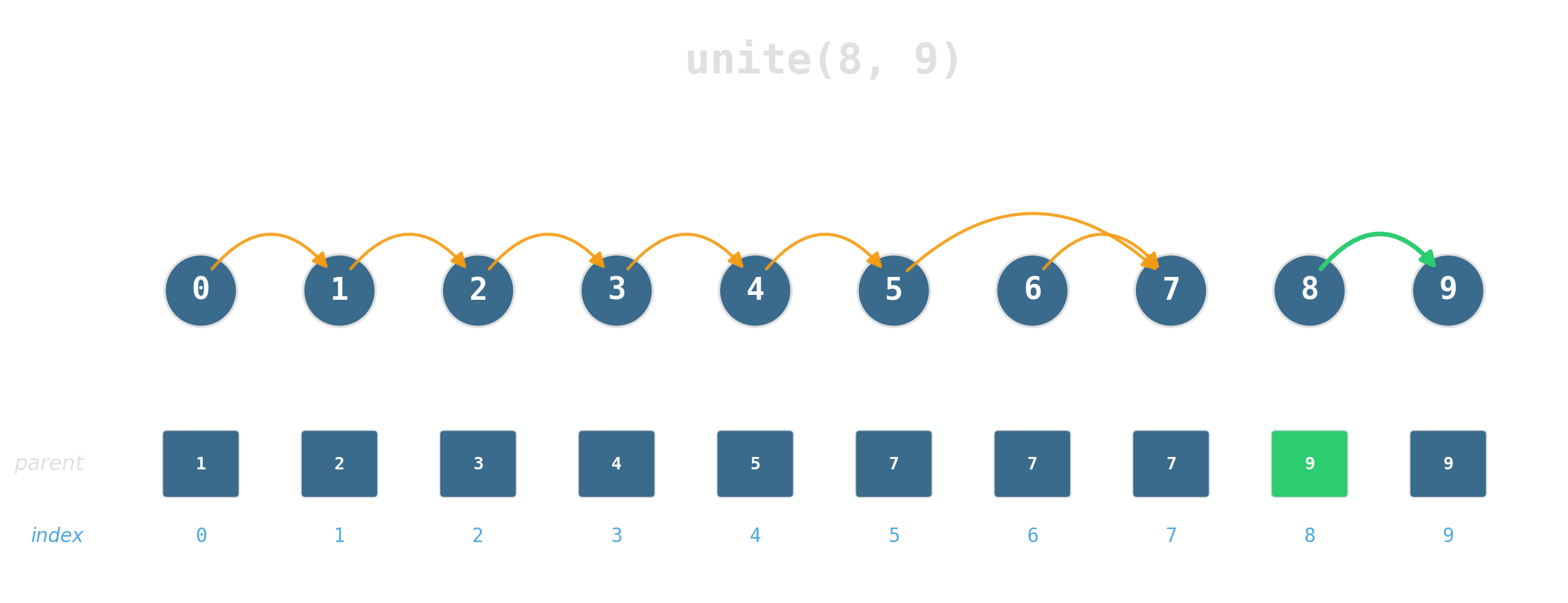
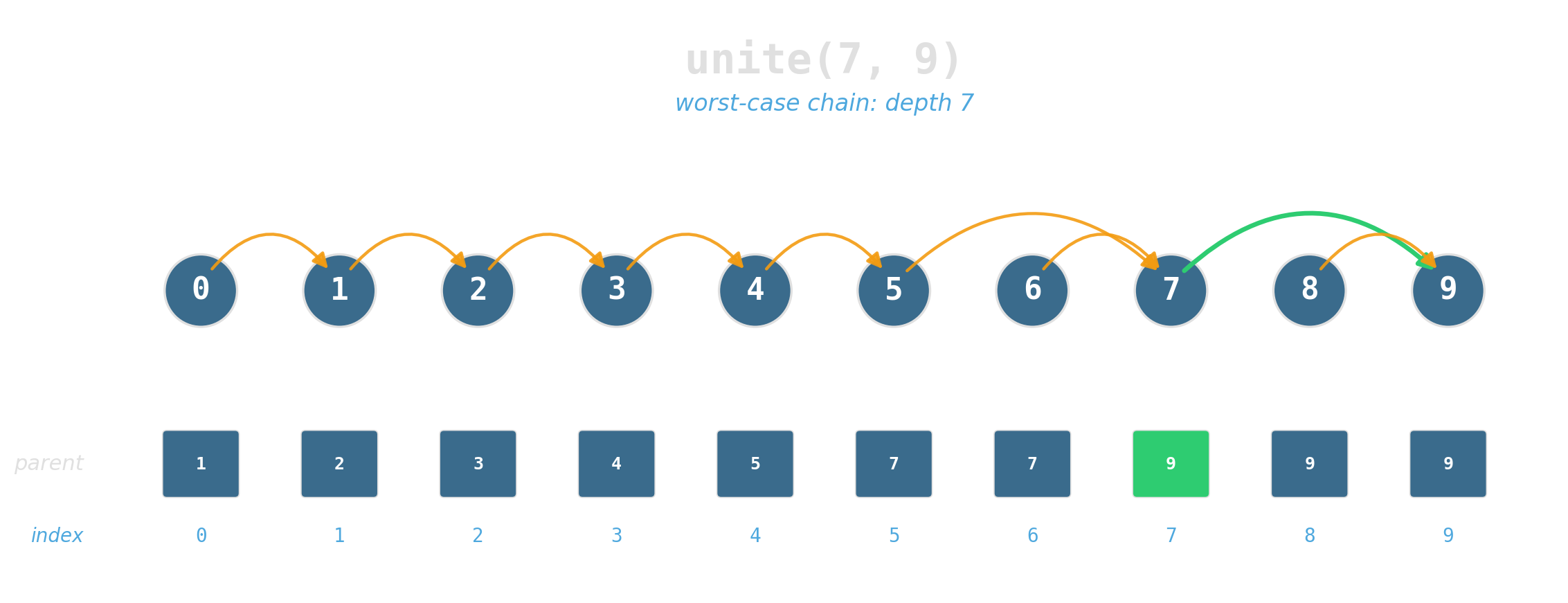
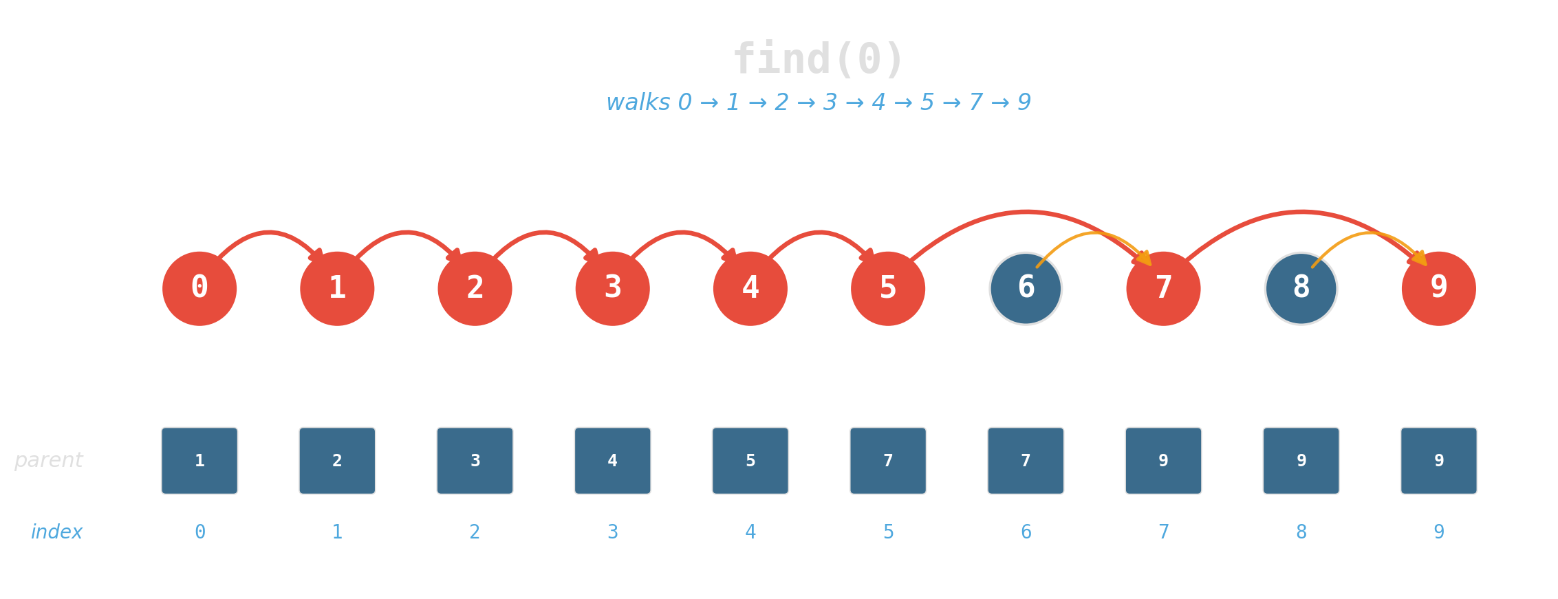
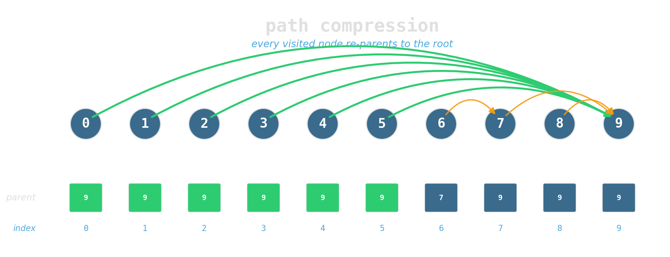
Union by rank: attach the shorter tree under the taller. Tree height stays logarithmic.

Path compression: during find, re-parent every node on the path directly to the root.

Twenty lines

#include <numeric>
#include <vector>

struct UnionFind {
    std::vector<int> parent, rank_;

    UnionFind(int n) : parent(n), rank_(n, 0) {
        std::iota(parent.begin(), parent.end(), 0);
    }

    int find(int x) {
        while (parent[x] != x) {
            parent[x] = parent[parent[x]];   // path halving
            x = parent[x];
        }
        return x;
    }

    void unite(int x, int y) {
        int rx = find(x), ry = find(y);
        if (rx == ry) return;
        if (rank_[rx] < rank_[ry]) std::swap(rx, ry);
        parent[ry] = rx;
        if (rank_[rx] == rank_[ry]) ++rank_[rx];
    }
};

Inverse Ackermann — and why it does not matter

Amortized cost per operation: \[O(\alpha(n))\]

For any n a physical computer can represent: α(n) ≤ 4.

In practice, treat both operations as O(1). The constant factor is dominated by the single cache line that holds the parent array hot.

Summary — union-find

Shape: a parent array, nothing else. Twenty lines of C++.
Tricks: union by rank, path compression (or halving) — apply both.
Cost: α(n) amortized; constant on any real input.
Spot it: dynamic partitions under merges, anywhere offline connectivity or equivalence classes appear.

Graphs

For graphs, the representation often matters as much as the algorithm.

Why graphs matter

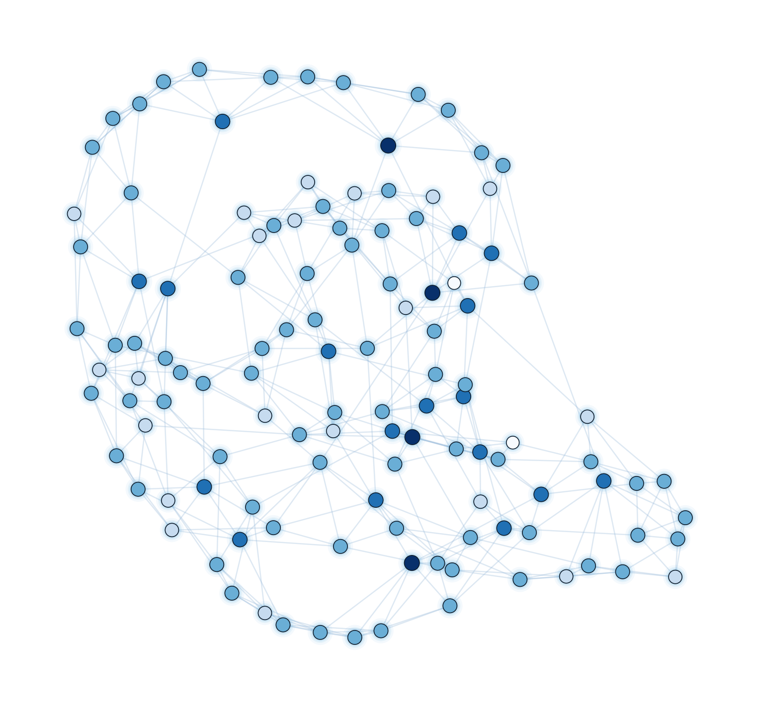
Graphs are arguably the dominant abstraction of combinatorial optimization.

They model concrete entities — people in a social network, intersections in a street network, machines on a factory floor.

…but just as naturally abstract ones — states of a system and the transitions between them, configurations of a puzzle, positions in a game.

Once a problem wears this shape, a huge library of algorithms becomes available. The rest of this chapter is about making those algorithms run fast on real hardware.

Compressed Sparse Row — two flat arrays

std::vector<std::vector<int>> places each vertex’s neighbors in a separate heap allocation: one cache miss per vertex before reading a single edge.

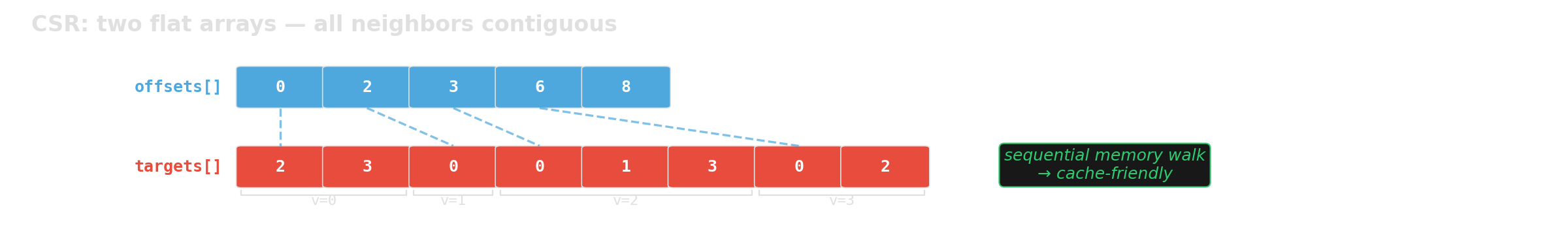
CSR is to graphs what std::vector is to linear structures — the default unless you have a specific reason otherwise.

Annotated graphs — where do weights live?

Per-vertex data (distance, parent, visited-flag): one parallel array per attribute, indexed by vertex id. Same pattern as std::vector<T>; no indirection.
Per-edge data on CSR: add a weights array of length E, aligned with targets. weights[i] is the weight of the edge whose target is targets[i]. Two parallel arrays become three; everything still streams.
AoS alternative: one struct Edge { int dst; float weight; } array. Better if the algorithm always touches both fields together; cache line carries what you need.

The annotation layout is the same AoS vs SoA question you already know. Fields the inner loop reads together should sit together; cold fields (labels, timestamps, provenance) go in their own array.

Adjacency matrix — when the graph is dense

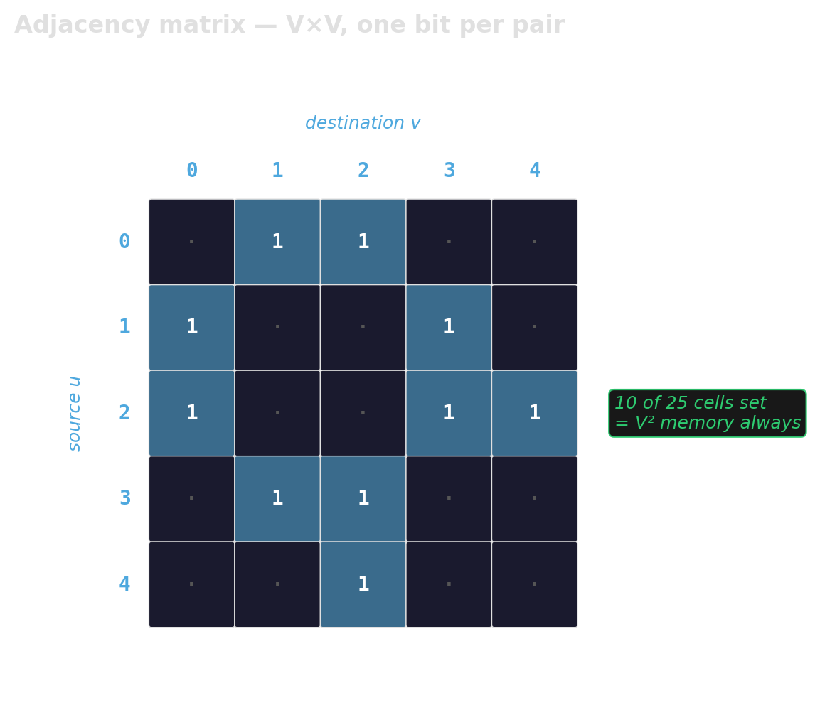
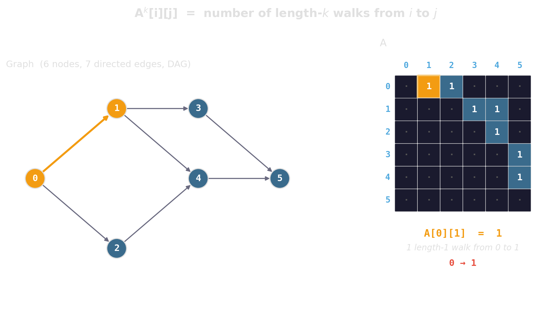
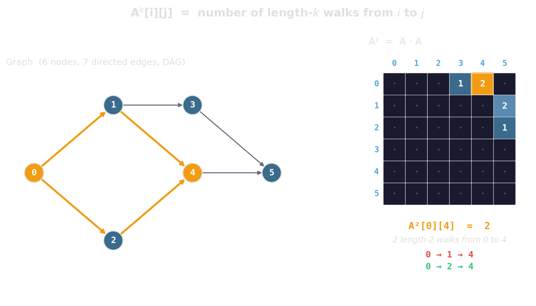
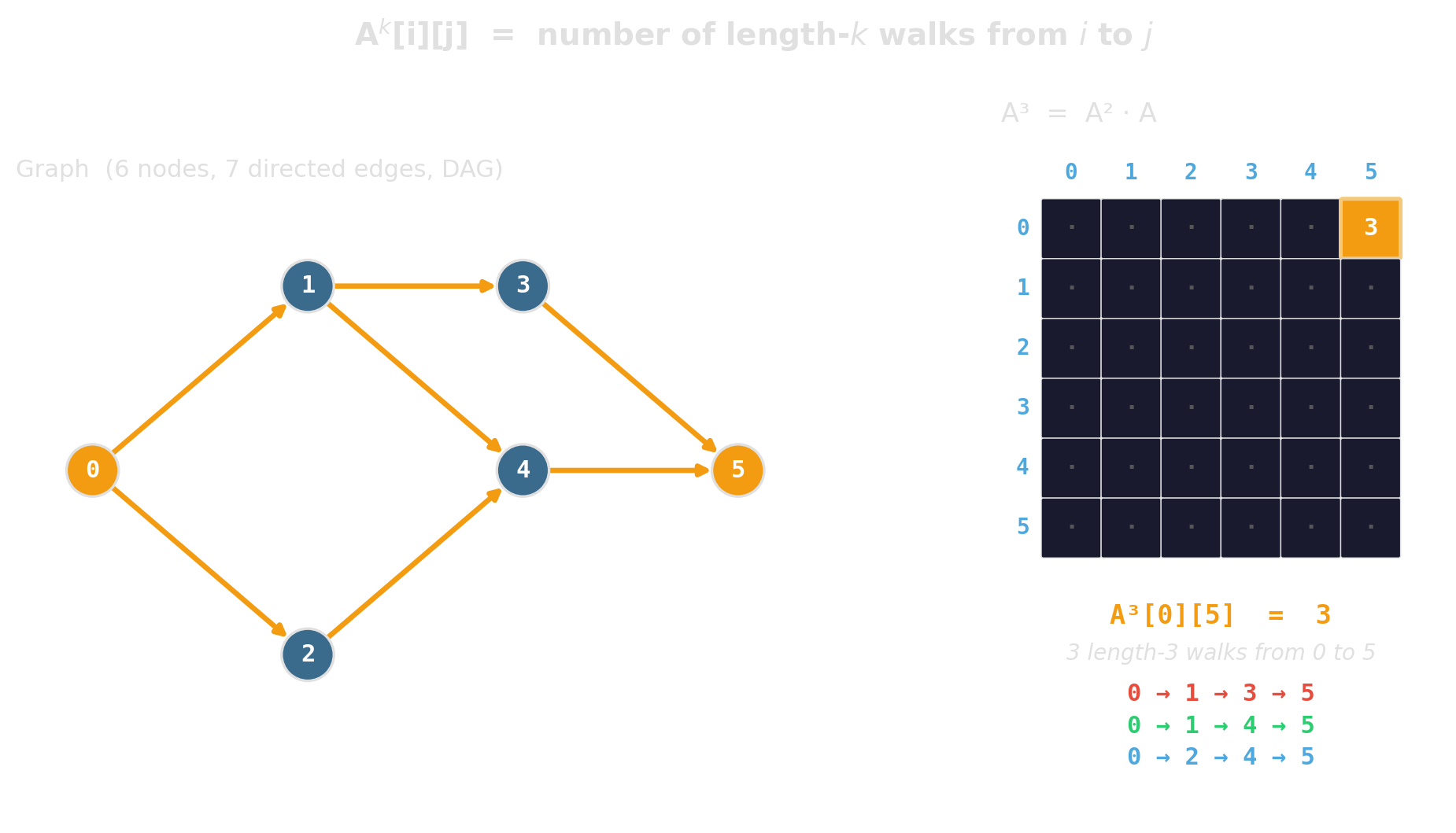
Right for small V with a dense graph, when edge-existence queries dominate, or when the algorithm is expressed as linear algebra (SpMV, matrix powers, GraphBLAS).

Bonus: the matrix is an algorithm

When the graph mutates

Pure CSR: fast reads, painful writes. Adding one edge shifts the rest.
Nested vector: cheap writes, slow reads.
In practice: keep a “cold” CSR snapshot plus a small “hot” delta structure. Rebuild periodically — every k inserts, or when the delta grows past some threshold.
Bulk loads: build an edge list, sort by source, convert to CSR in one pass.

Summary — graphs

Default: CSR. Two flat arrays, streams at memory bandwidth.
Avoid: std::vector<std::vector<int>> as a long-lived representation — same pathology as std::list.
Edge-centric: an edge list, sorted as the algorithm needs.
Dynamic: CSR plus a small delta, rebuild periodically.

Spatial Data Structures

Queries in space, not by key. That usually calls for different structures.

When do we need them?

Too many geometric objects to scan: millions of points, rectangles, triangles, particles.
Queries are local in space: near-neighbor, range, ray/intersection, or collision — only a small region is relevant.
Most data is irrelevant per query: the whole win comes from pruning almost everything.
Everywhere: GIS/maps, game physics, robotics, CAD, ray tracing, nearest-neighbor search.

The structure is chosen by the query, not the data. Range → grid/R-tree. Nearest-neighbor → kd-tree. Ray → BVH. Collision → BVH/grid. The rest of this section is a menu.

Uniform grid — the boring, often-winning baseline

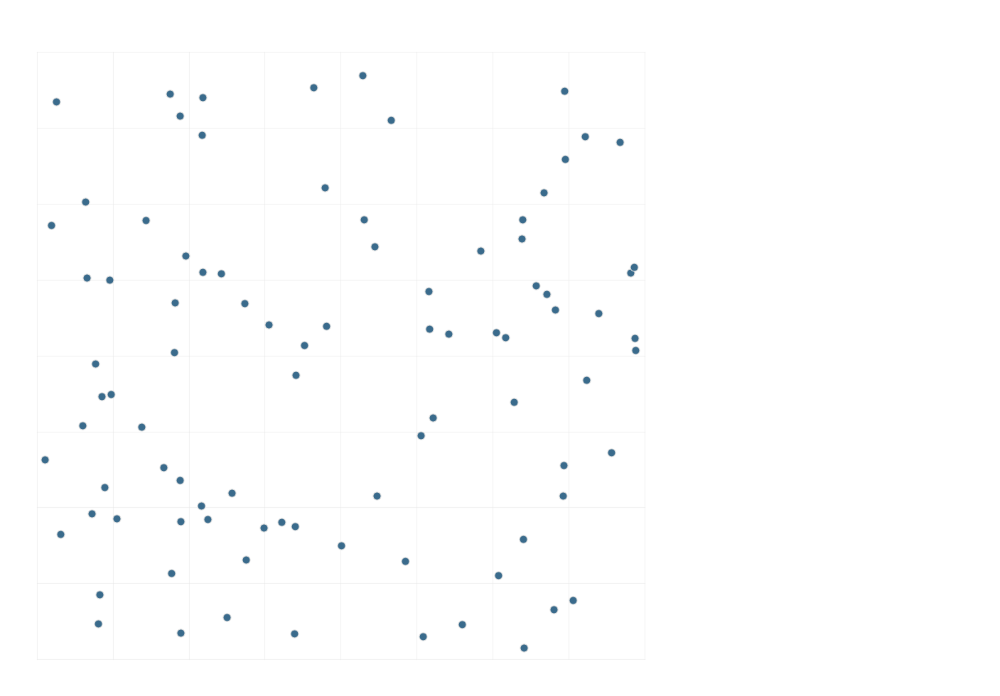
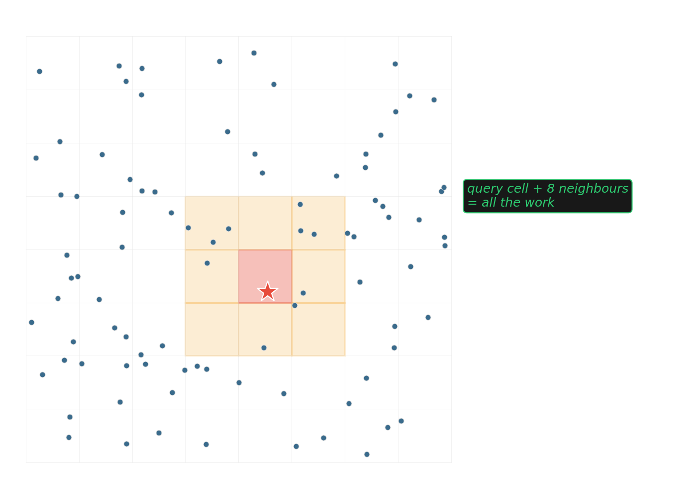
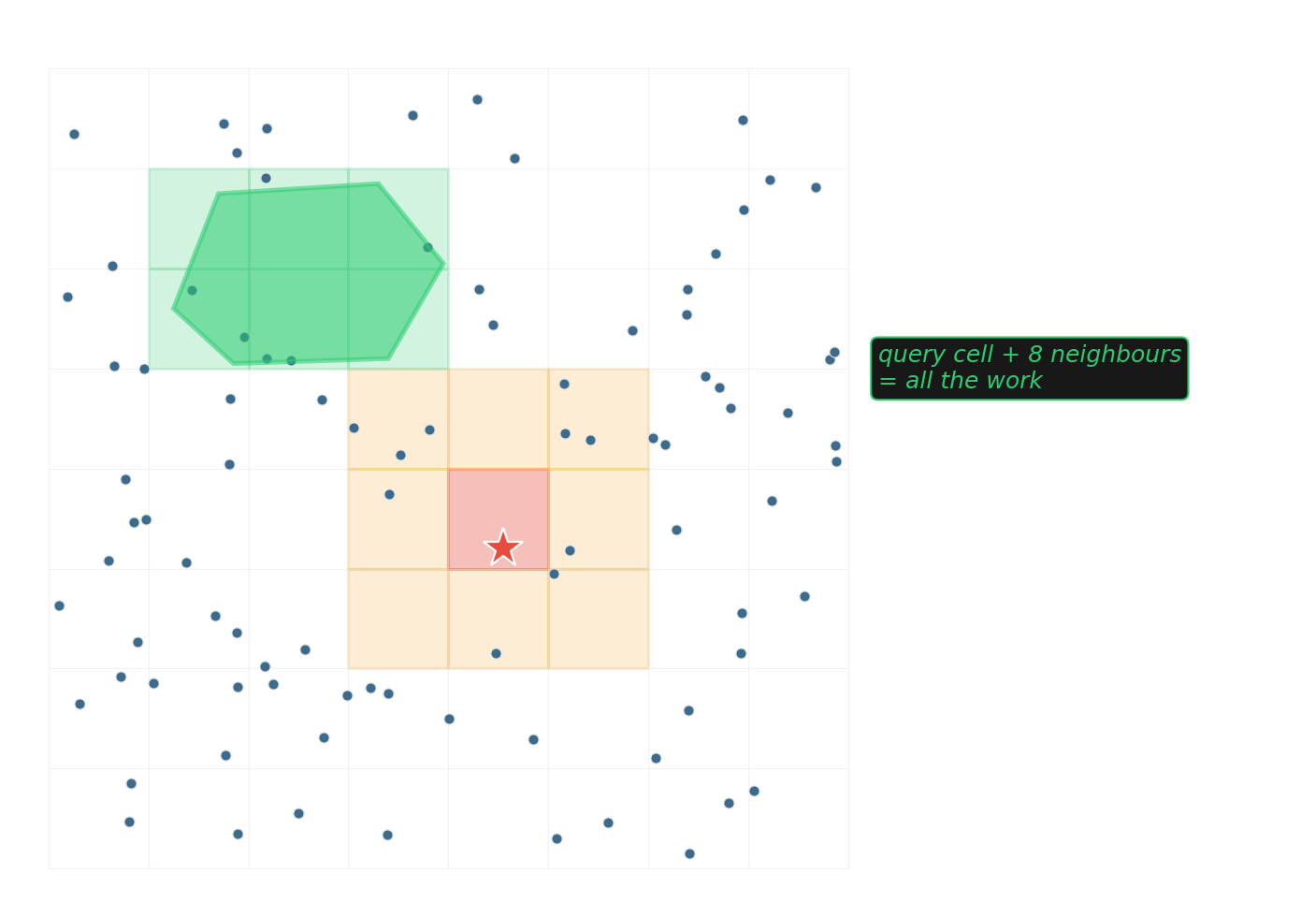
\(O(1)\) expected for near-neighbor queries when points are roughly uniform. One array of bucket vectors, one divide-and-floor to find a cell.

kd-tree — recursive median splits

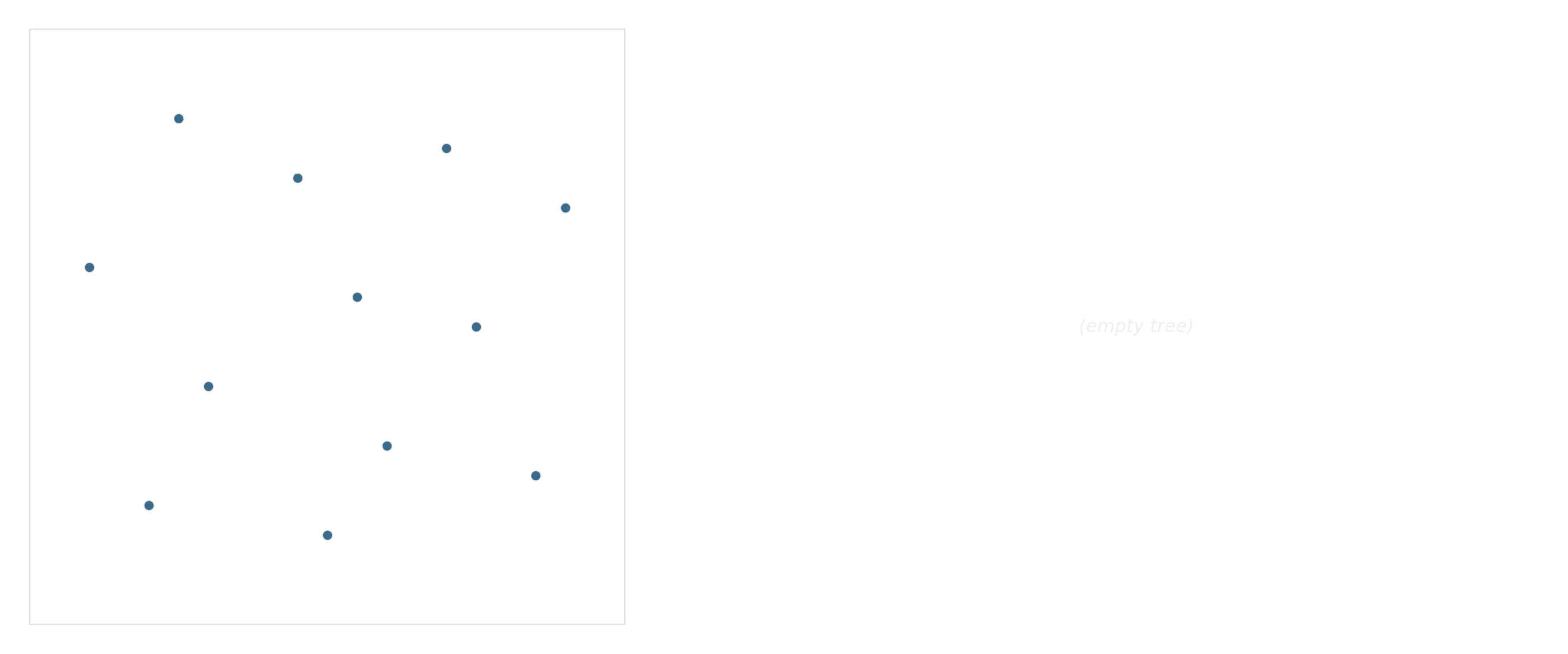
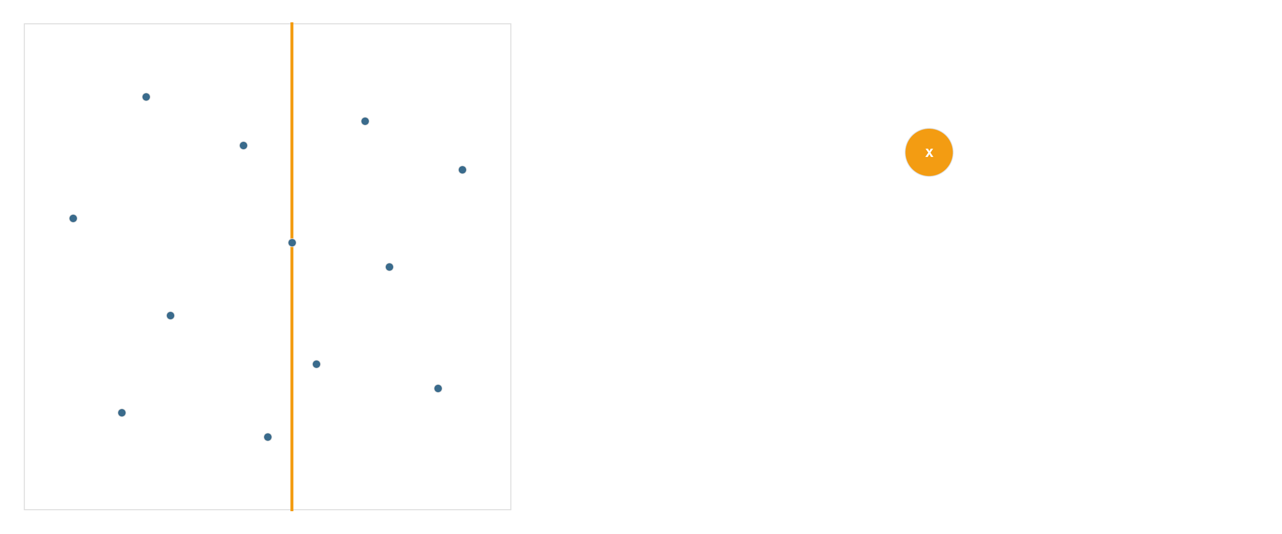
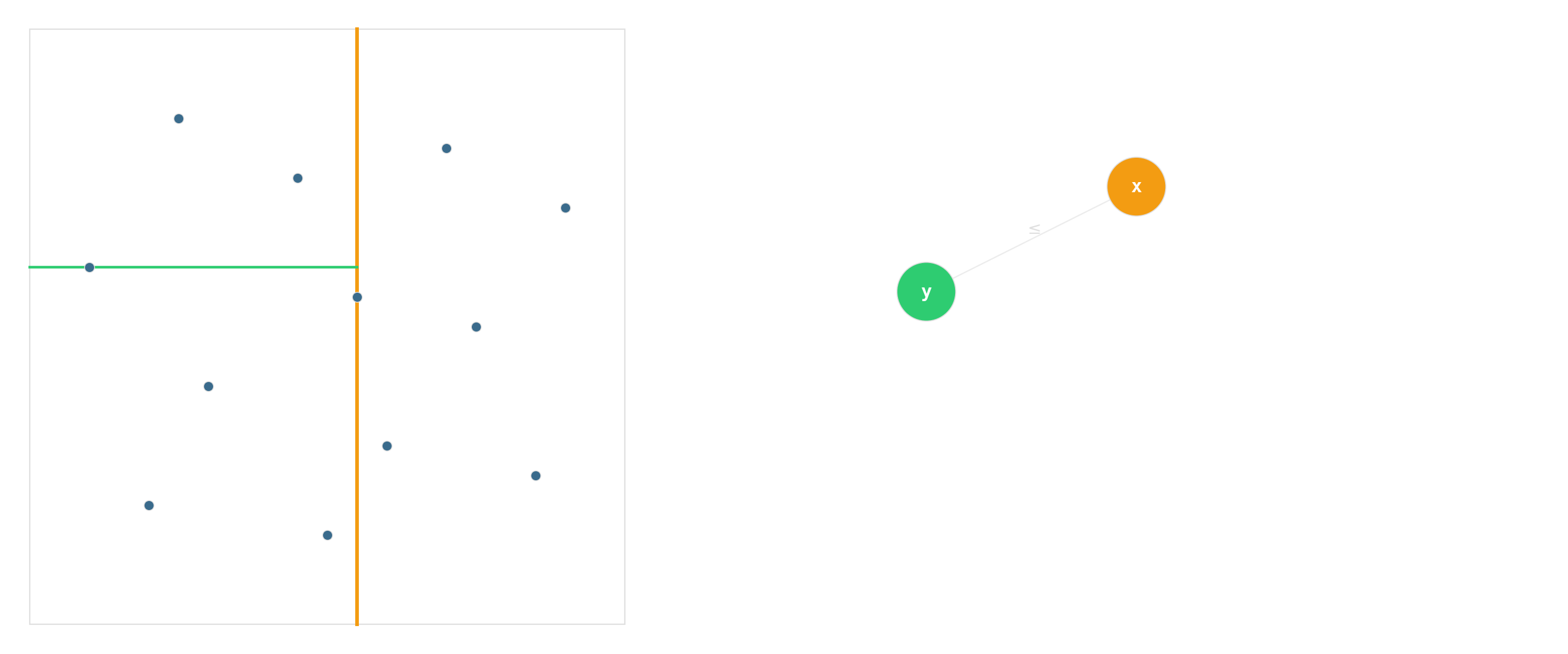
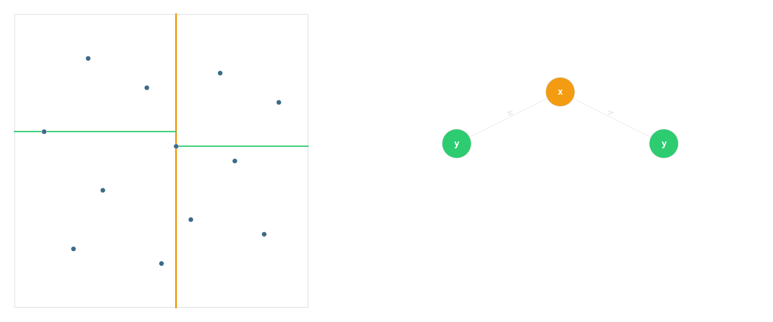
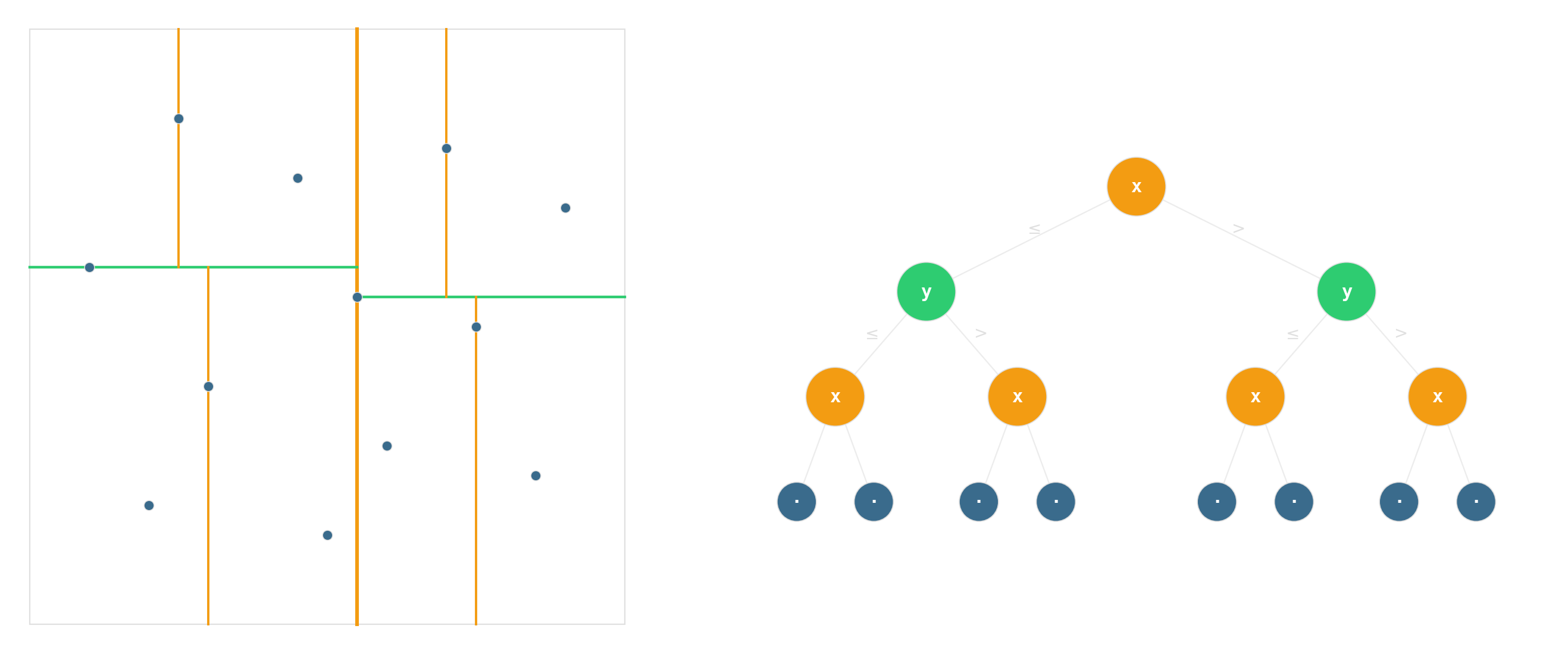
Degrades to linear scan as dimensionality rises. By about twenty dimensions, brute-force is competitive. This is the “curse of dimensionality” for data structures.

BVH — the ray-tracing workhorse

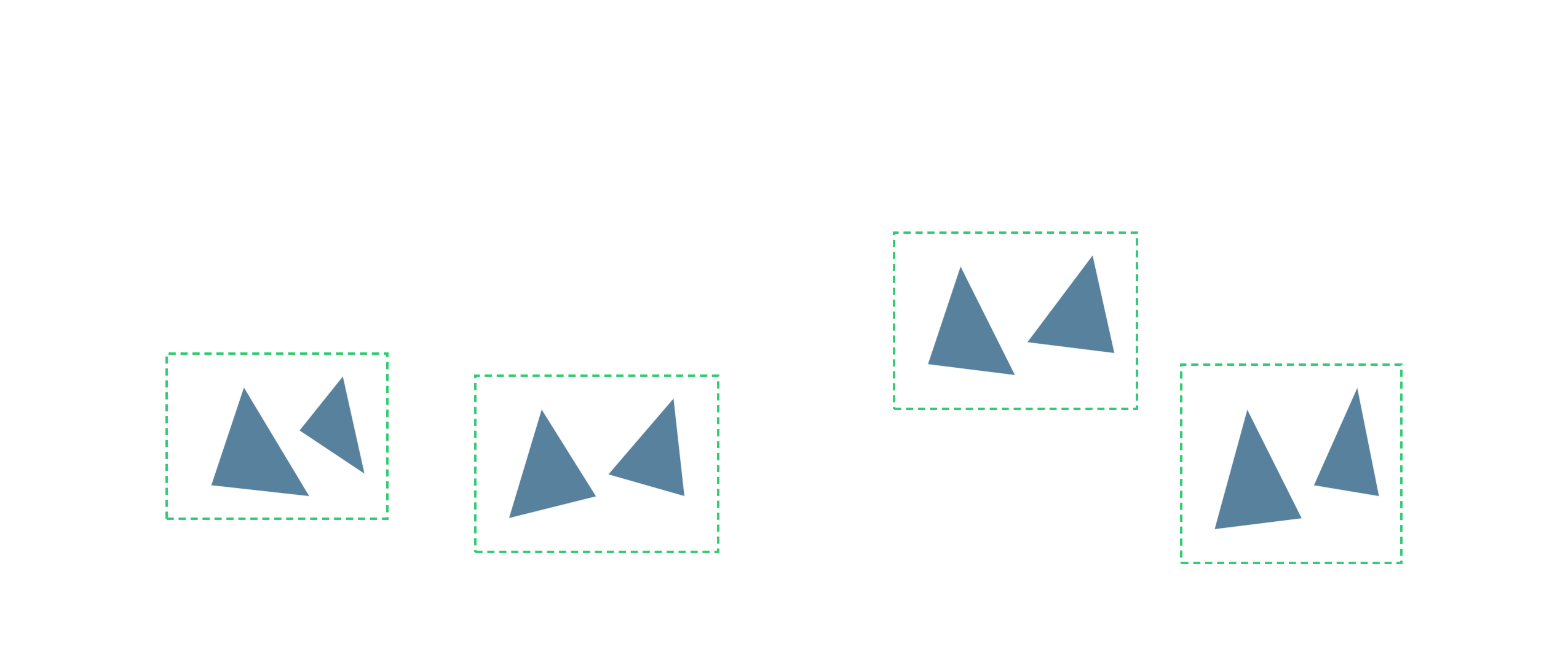
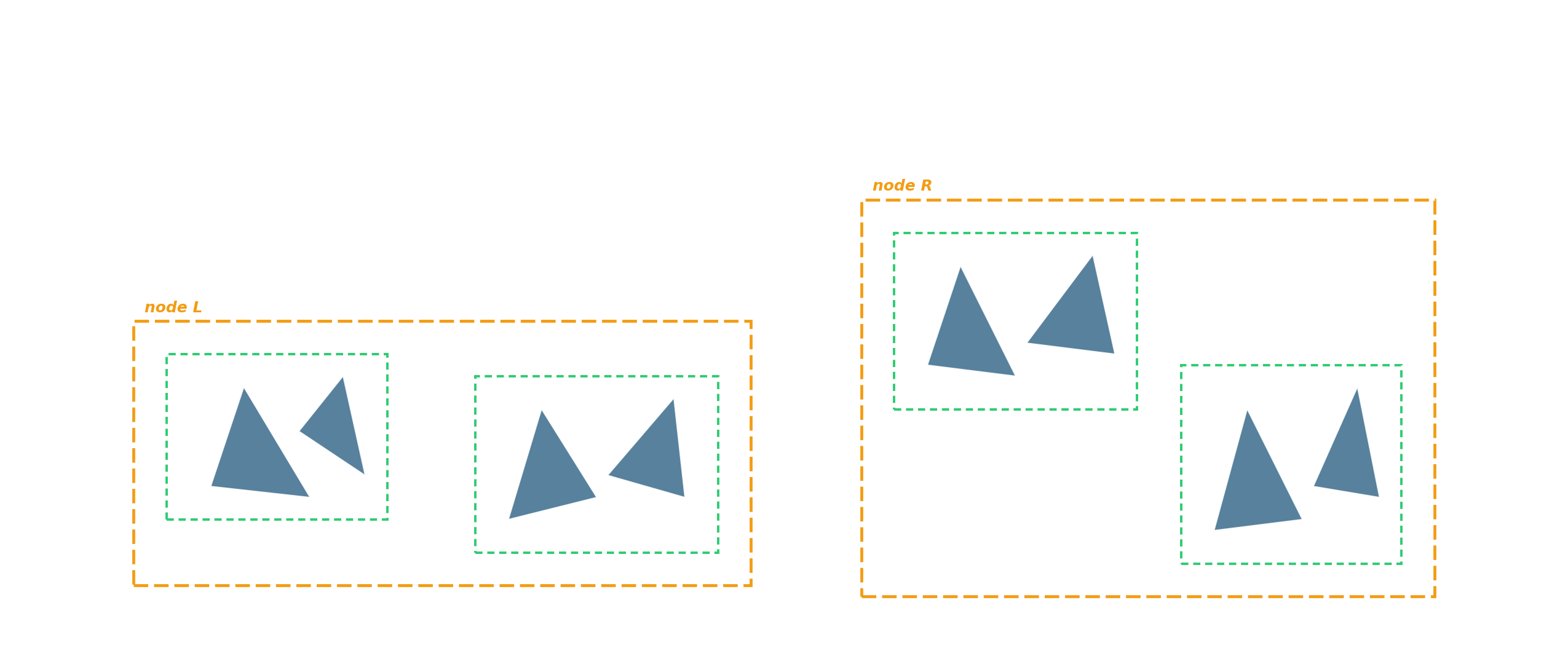
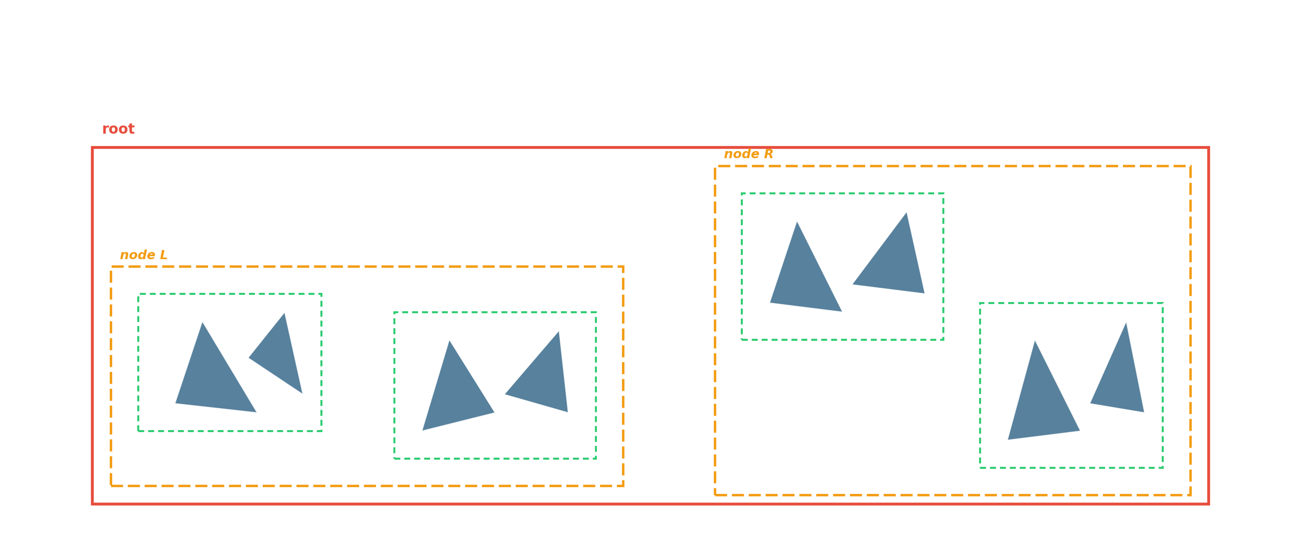
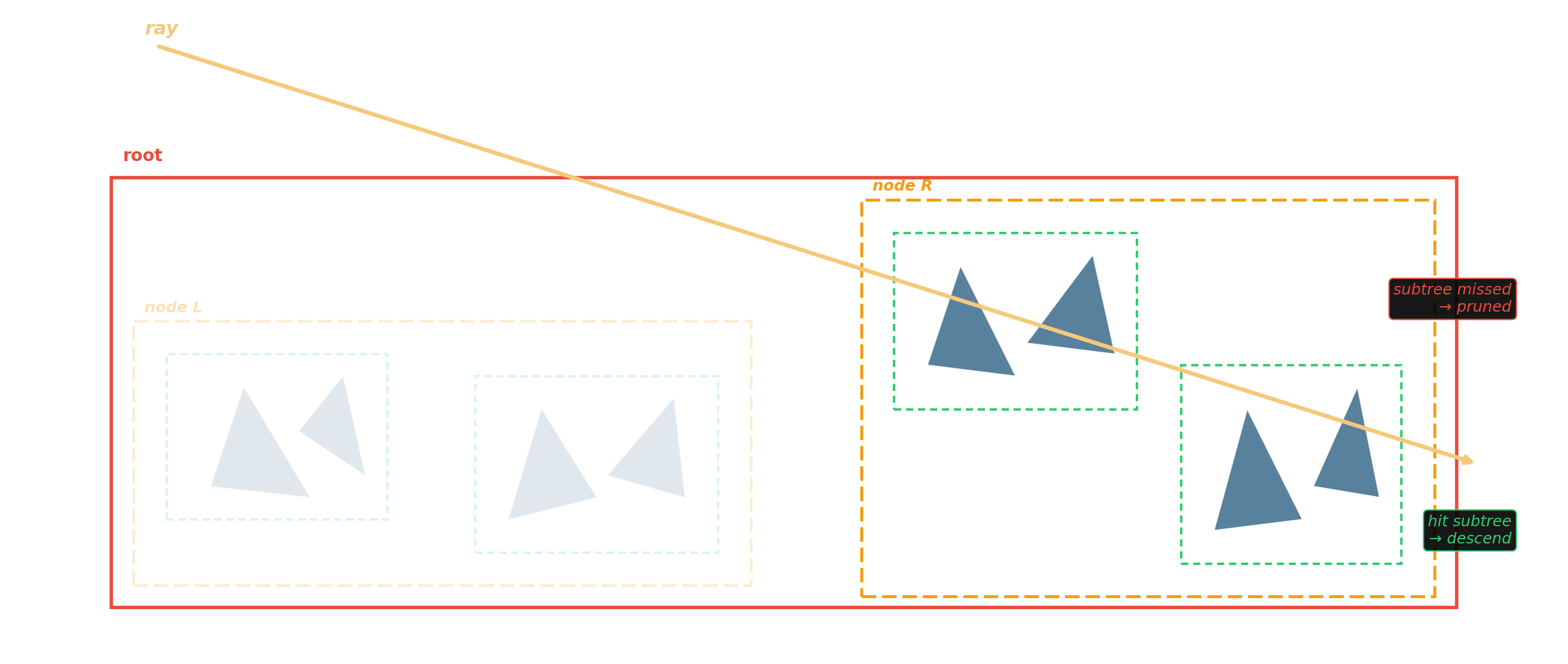
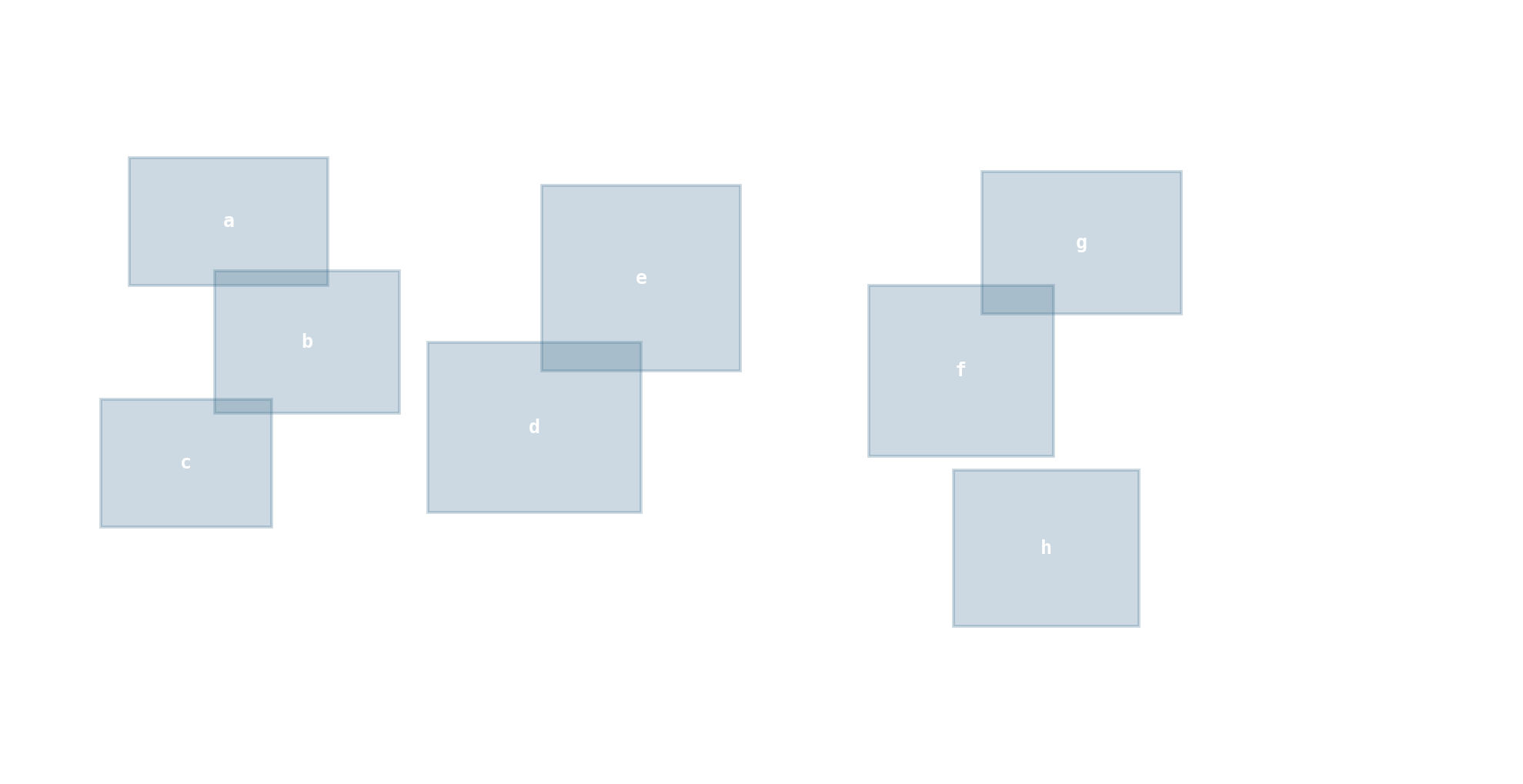
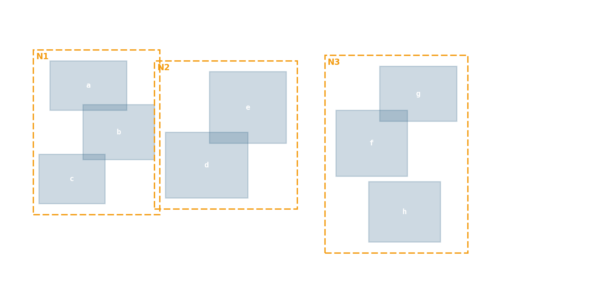
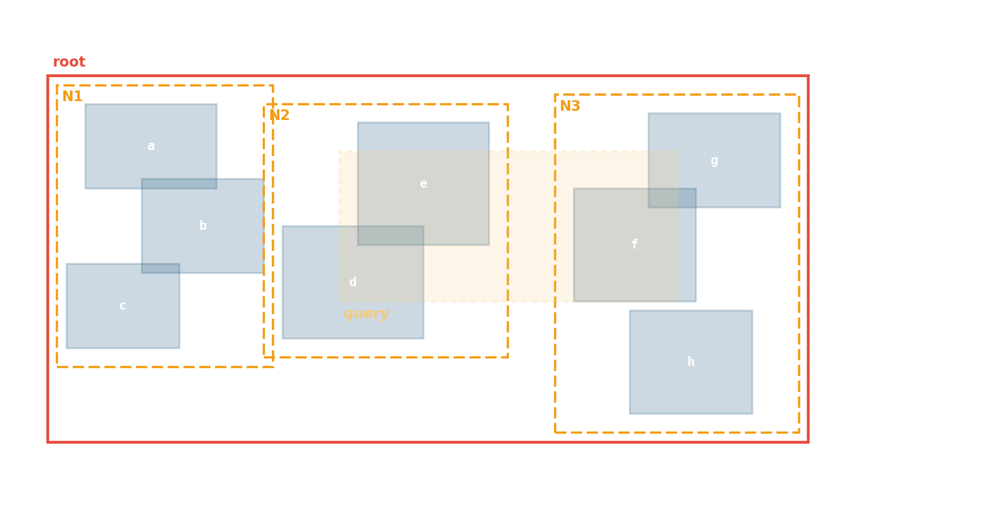
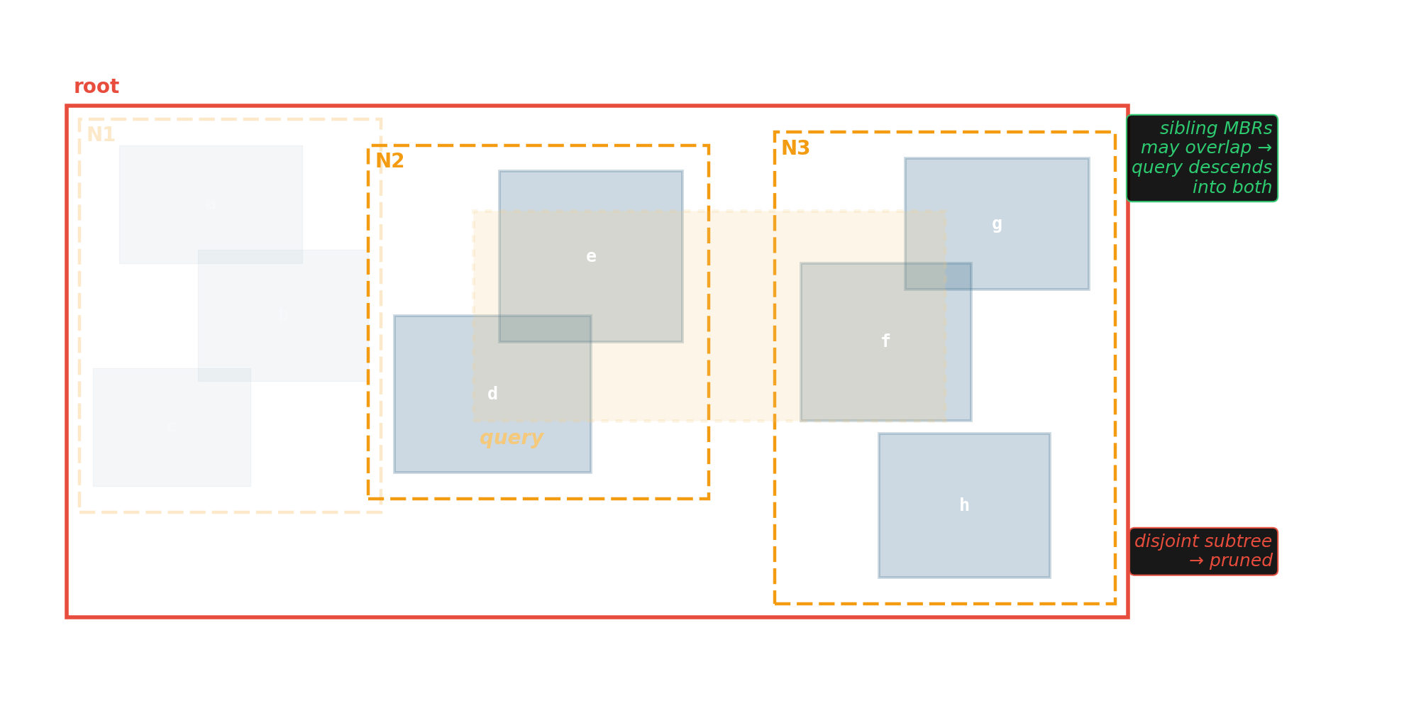
R-tree — rectangles in a database

Delaunay triangulation — geometry → sparse graph

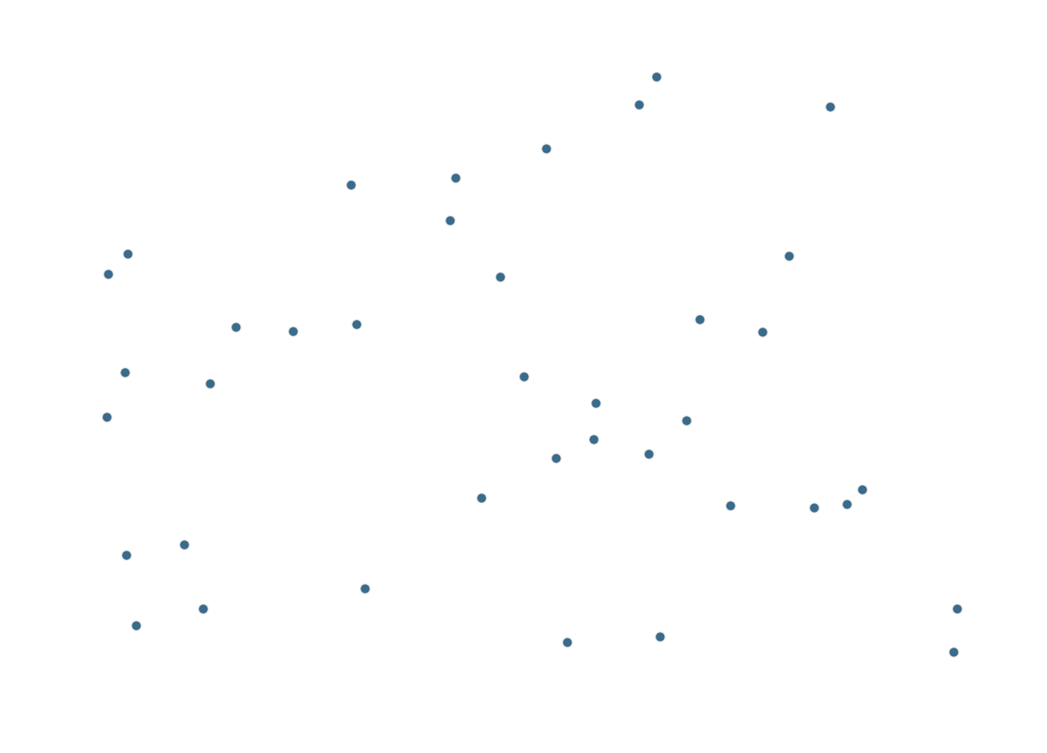
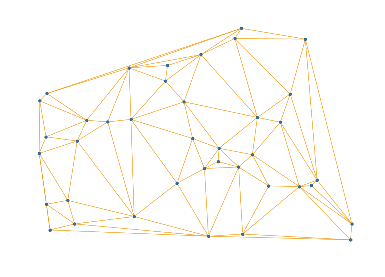
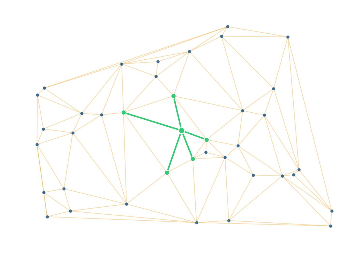
Not a query accelerator — a graph builder. Turns a point cloud into a sparse planar graph so downstream graph algorithms have something to walk.

Summary — spatial structures

Default for points: uniform grid. Simple, fast, often enough.
Low-D nearest neighbor: kd-tree. Degrades above ~10 dimensions.
Objects, rays, collisions: BVH. Build quality dominates traversal speed.
On-disk rectangles: R-tree.
Sparse proximity graph: Delaunay triangulation — bridge to graph algorithms.
High-D embeddings: approximate methods — a topic of its own.

Probabilistic Structures

A closing party trick: give up exactness for tiny memory — simple, surprising, rarely taught.

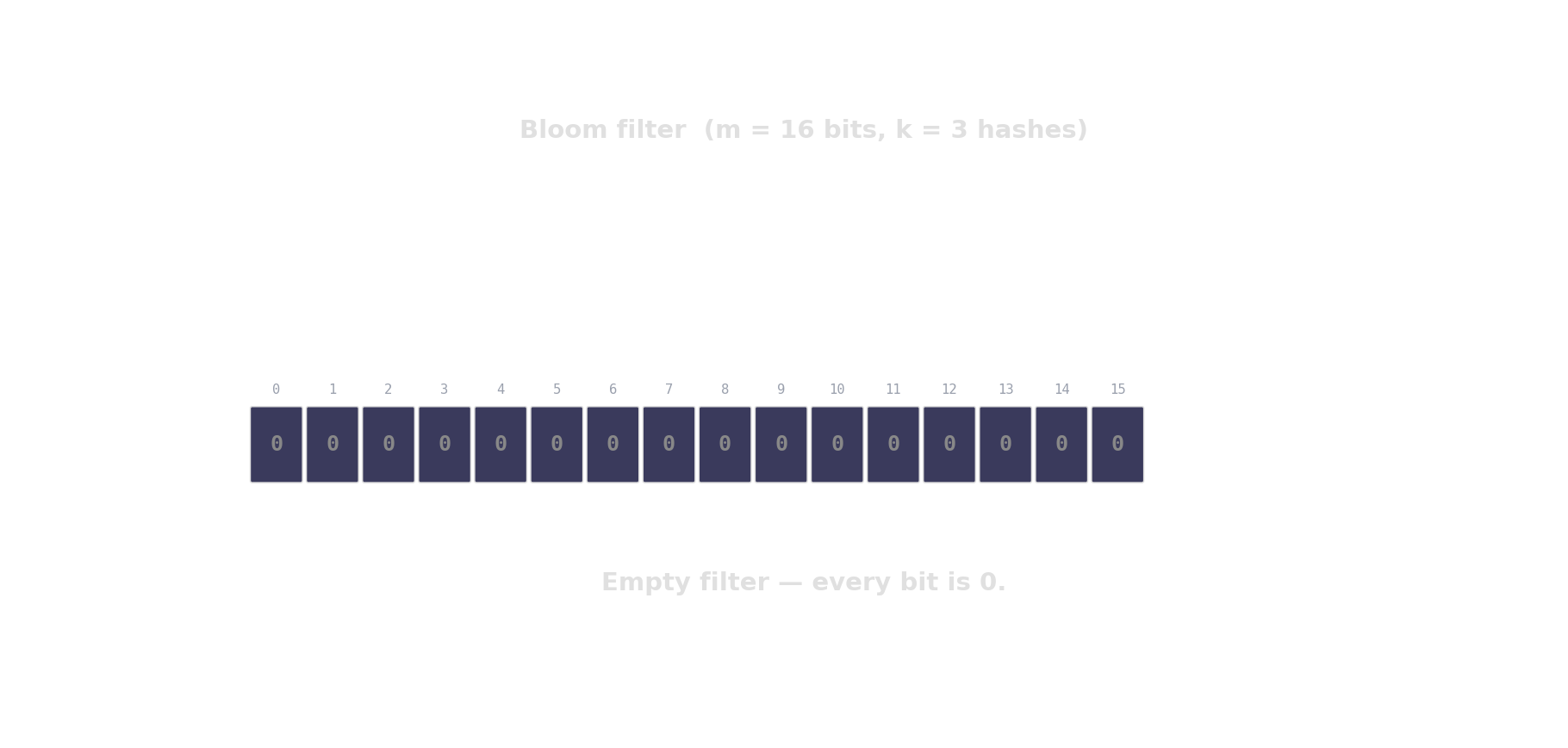
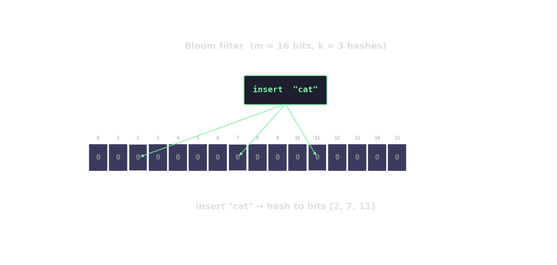
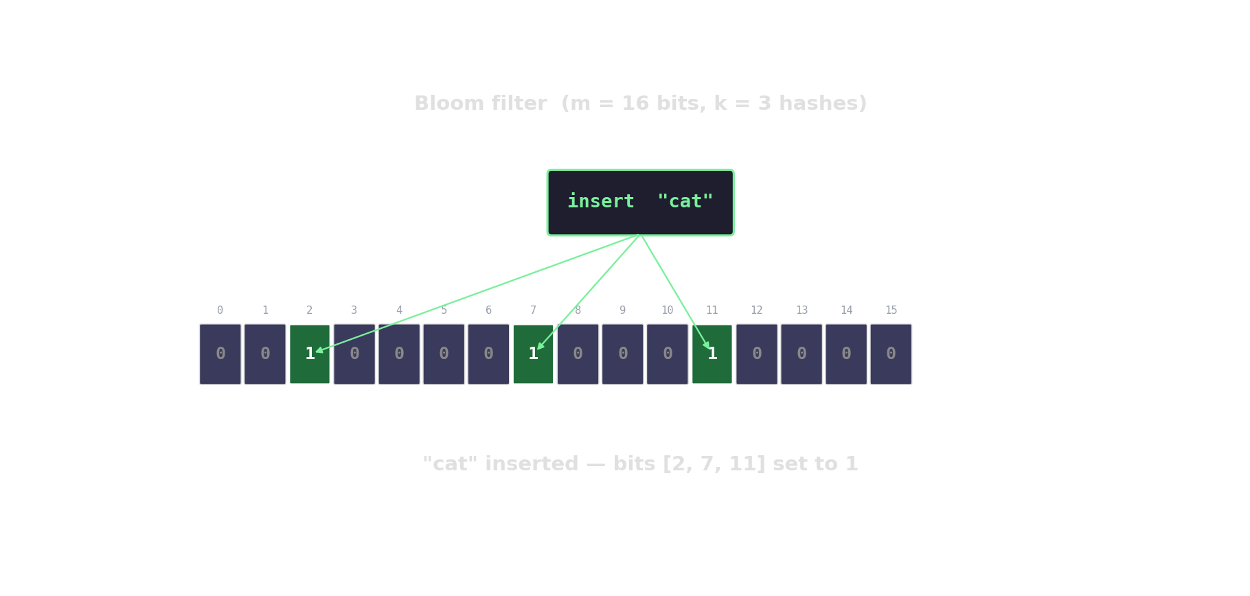
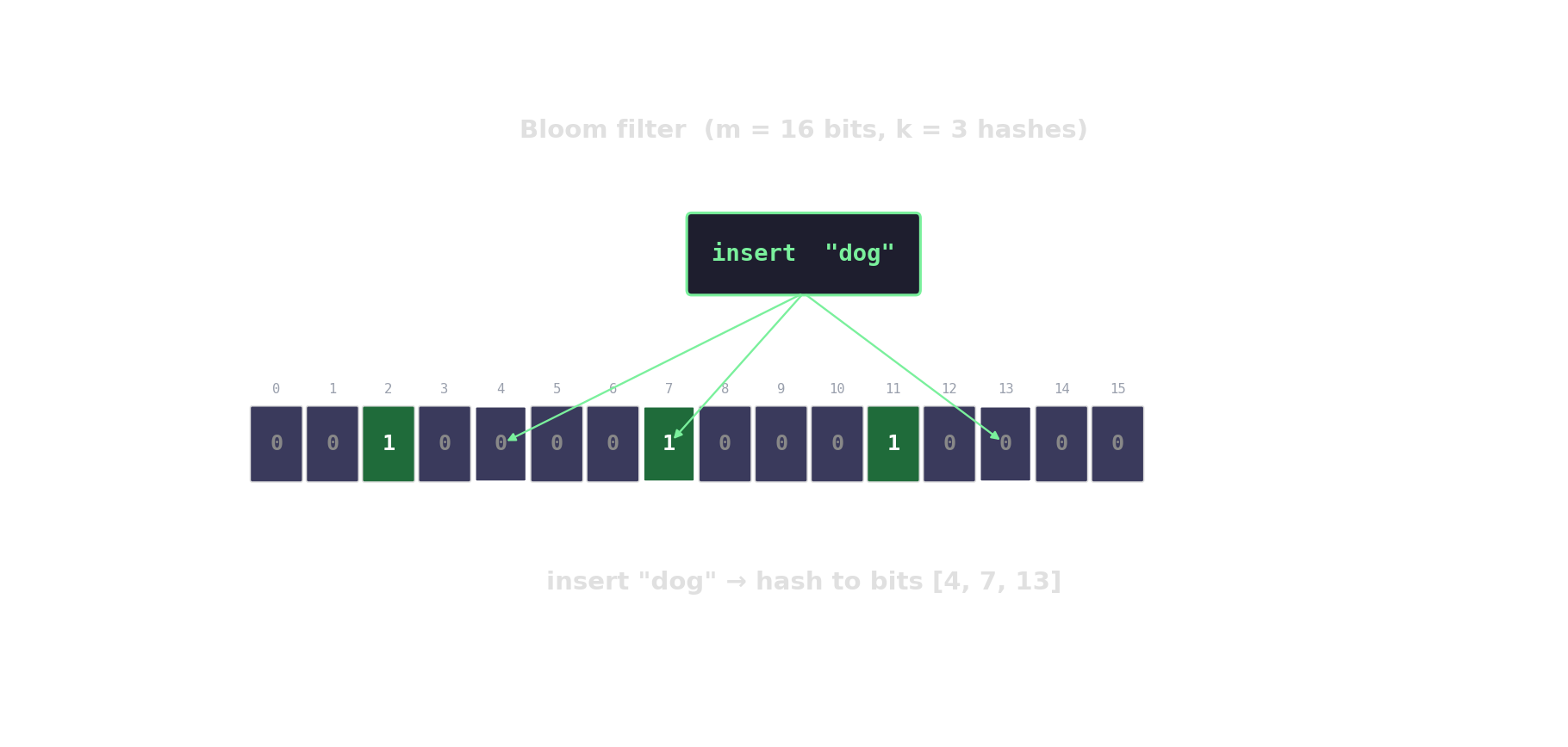
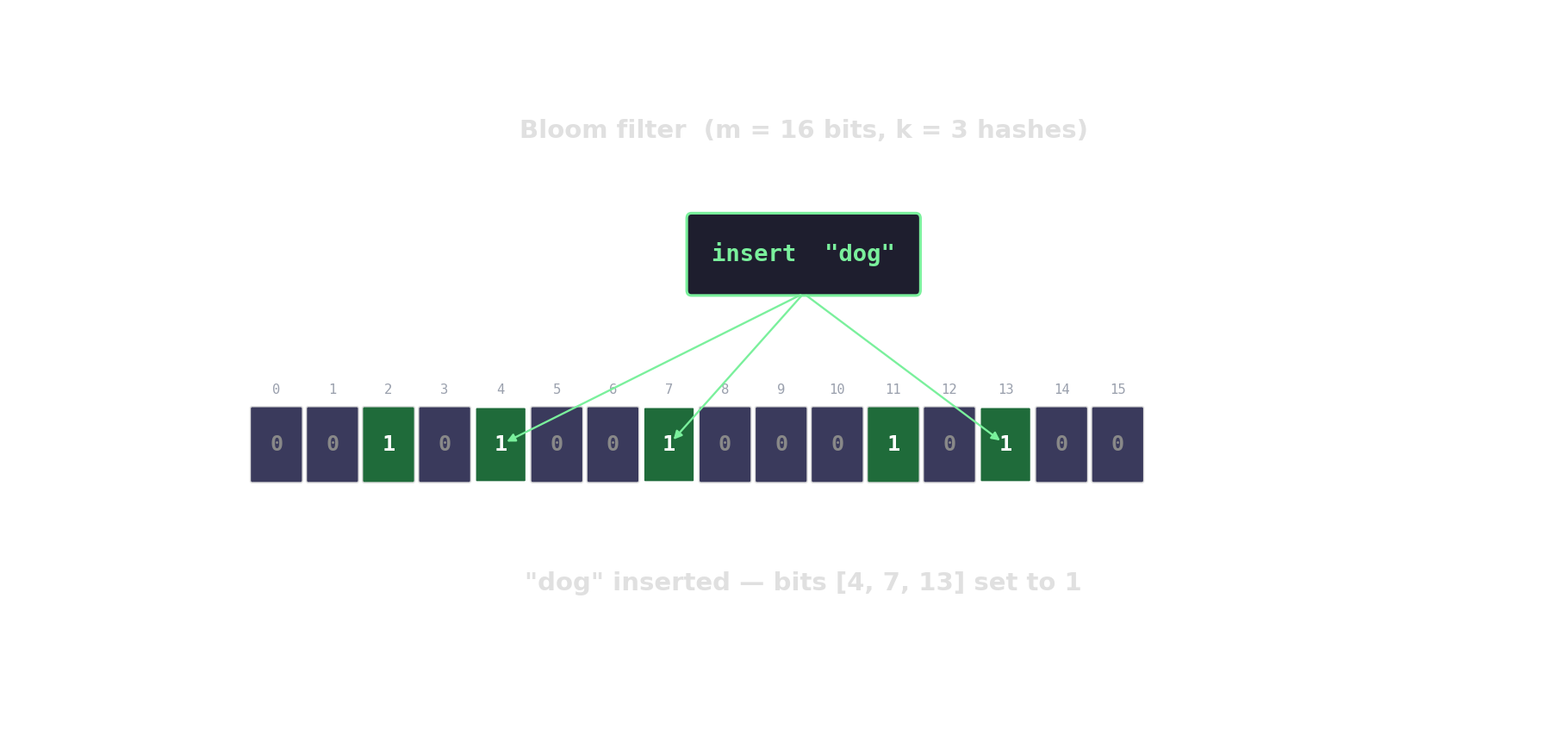
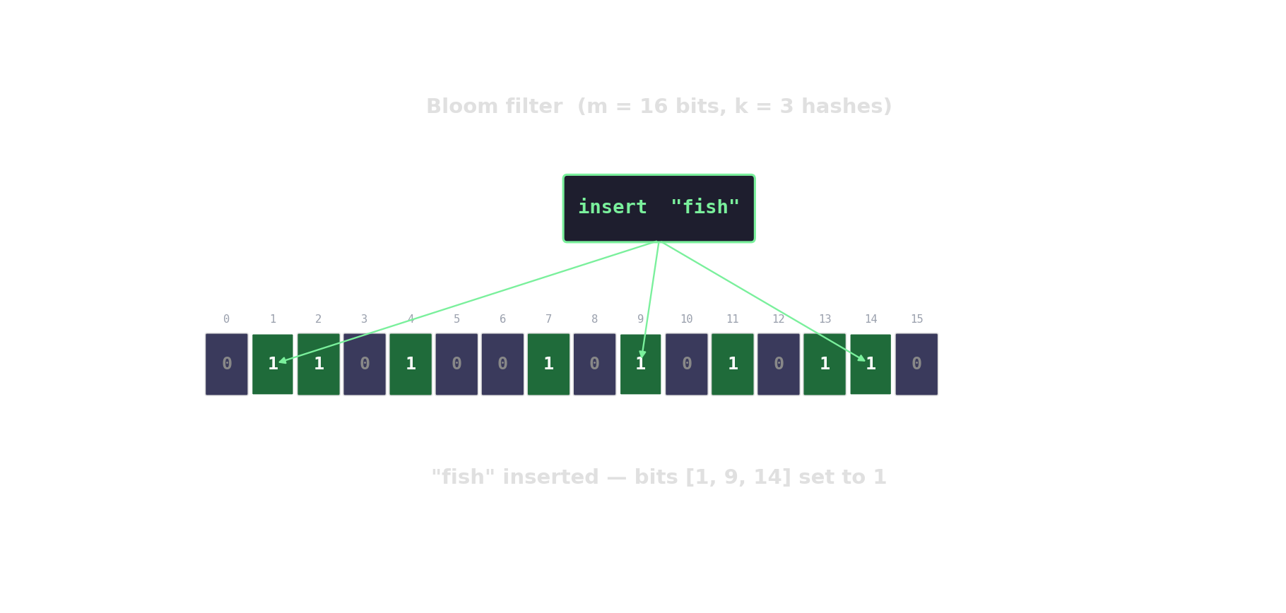
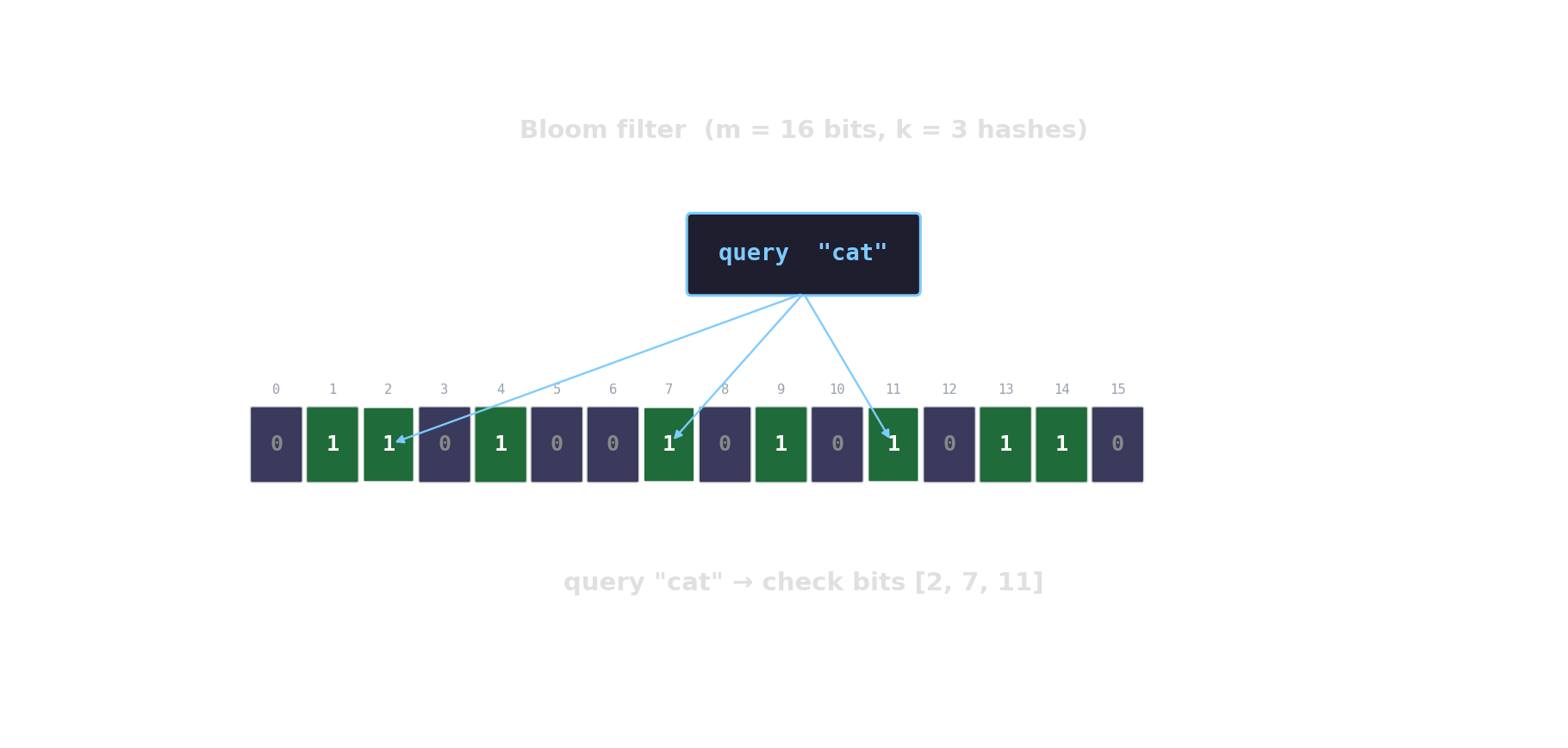
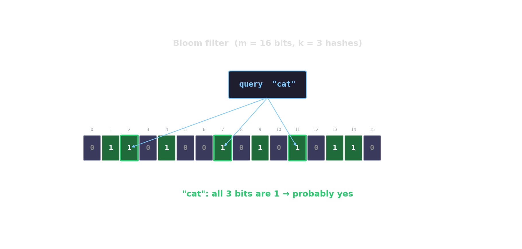
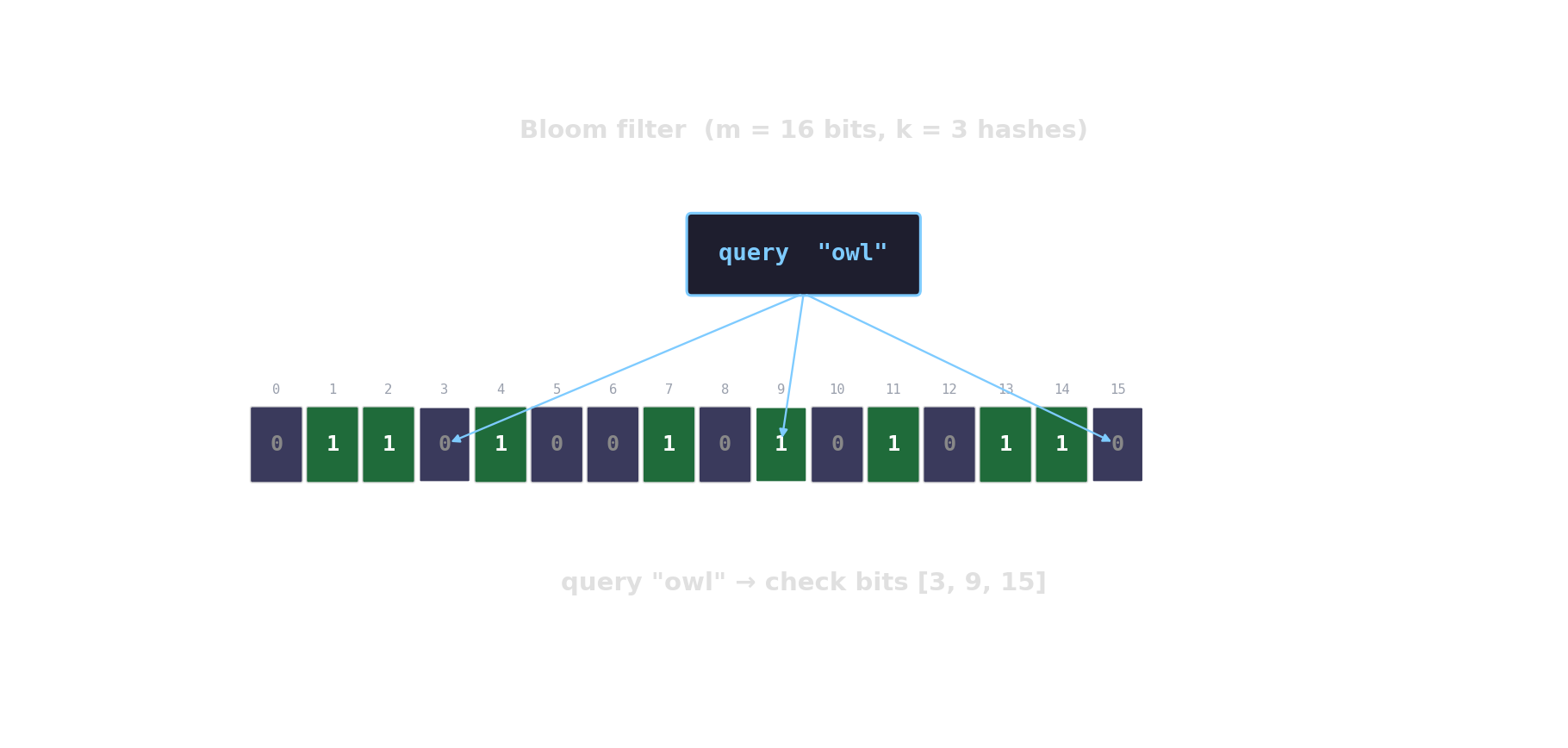
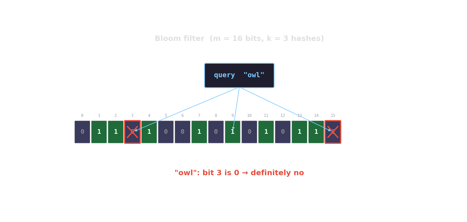
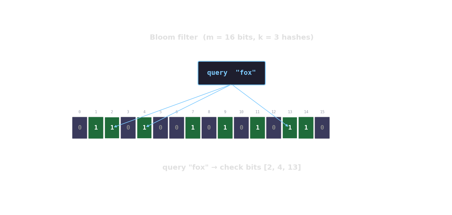
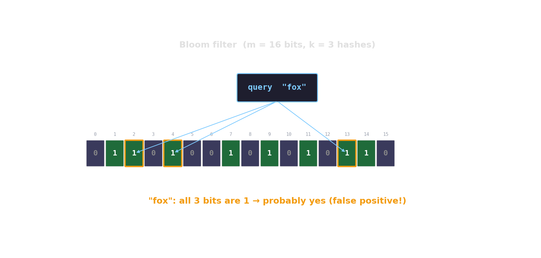
Bloom filter in action

Where does the false-positive rate come from?

\[\Pr[\text{a fixed bit stays 0 after one hash}] \;=\; 1 - \tfrac{1}{m}\]

\[\Pr[\text{it stays 0 after all } kn \text{ hashes}] \;=\; \left(1 - \tfrac{1}{m}\right)^{kn} \;\approx\; e^{-kn/m}\]

\[\Pr[\text{bit is 1}] \;\approx\; 1 - e^{-kn/m}\]

\(m\): size of bit array

\(k\): number of hashes

\(n\): inserted elements

A non-member query hits \(k\) bits independently — false positive iff all are 1: \[\Pr[\text{false positive}] \;\approx\; \left(1 - e^{-kn/m}\right)^{k}\]

Minimize over \(k\) for fixed \(m/n\): optimum at \(k^\star = \tfrac{m}{n}\ln 2\).

Sizing a Bloom filter in practice

bits / element	optimal \(k\)	FPR	for \(n = 10{,}000{,}000\)
4	3	14.7 %	4.8 MB
6	4	5.6 %	7.2 MB
8	6	2.2 %	9.5 MB
10	7	0.82 %	12 MB
12	8	0.31 %	14 MB
16	11	0.046 %	19 MB
20	14	0.0068 %	24 MB

Rule of thumb: each ~5 bits per element buys roughly a 10× lower FPR. Ten bits (~1 %) is the default most libraries pick; go higher only when a false positive is genuinely expensive.

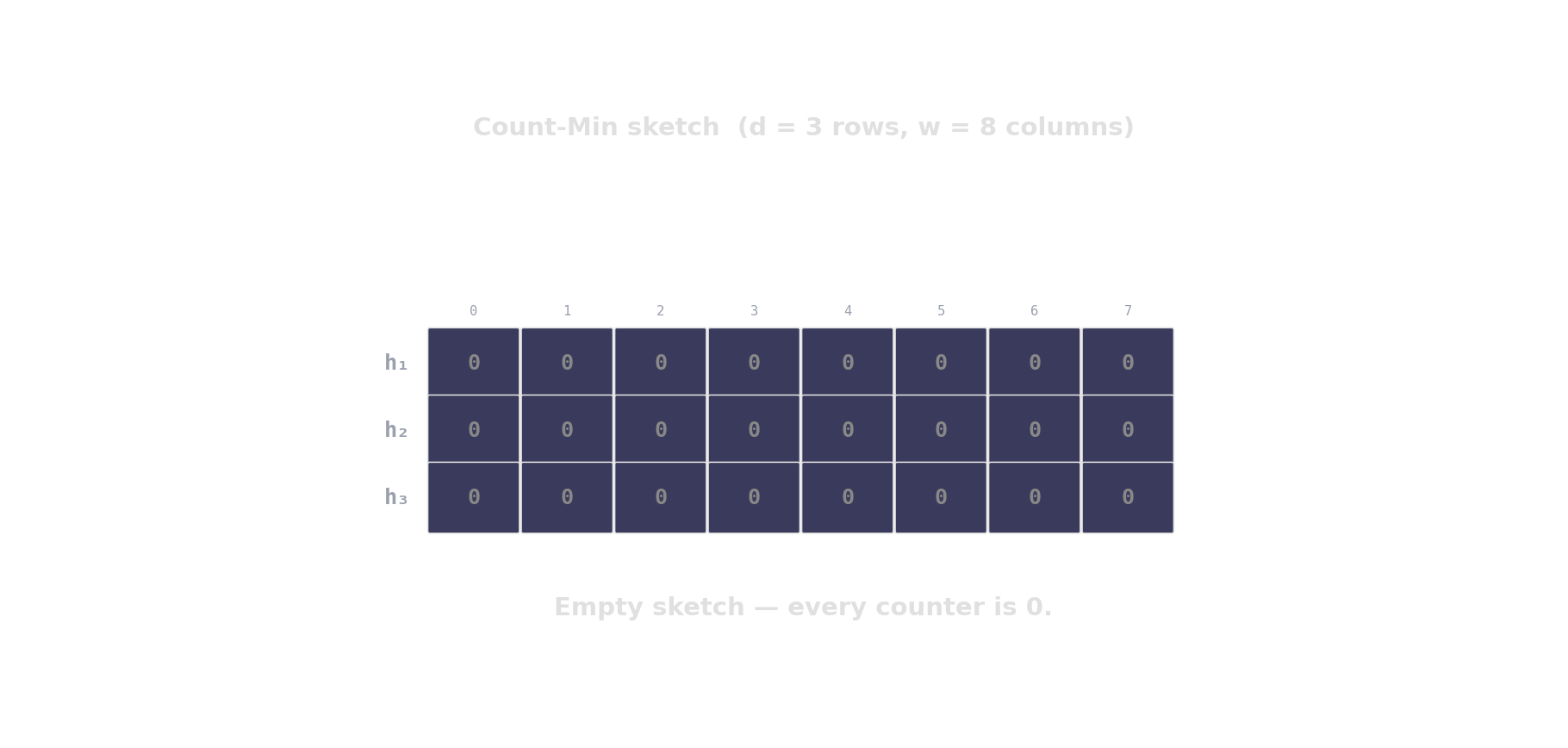
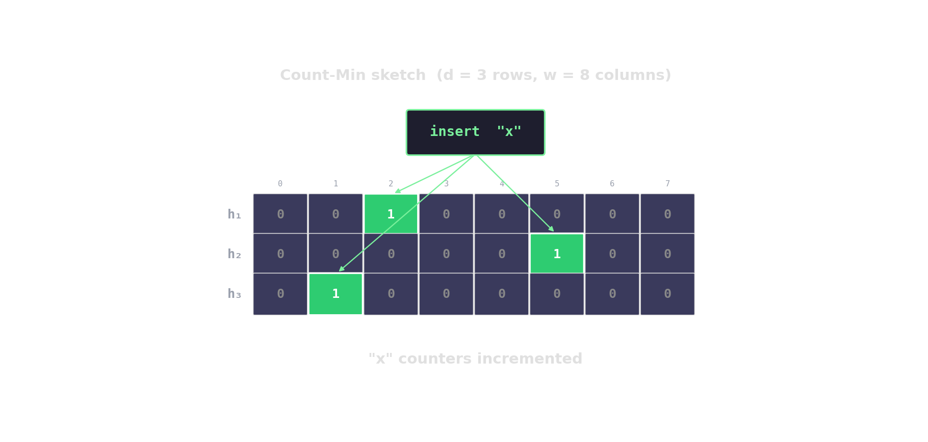
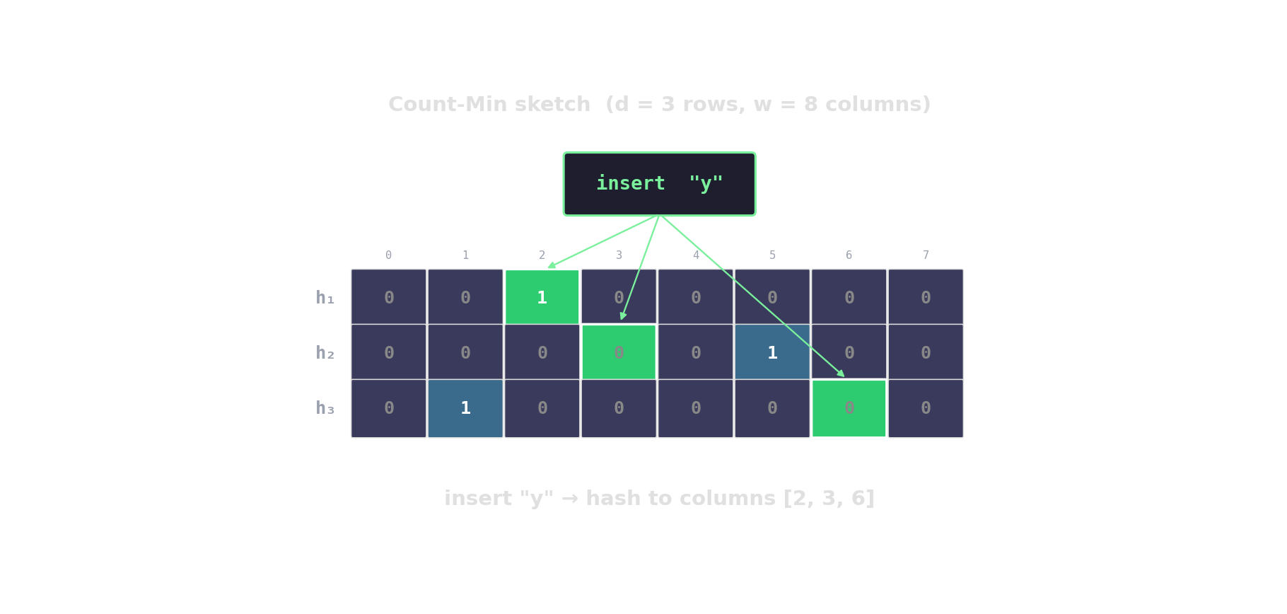
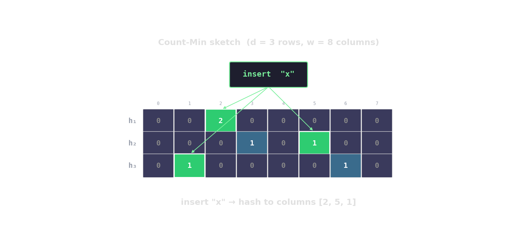
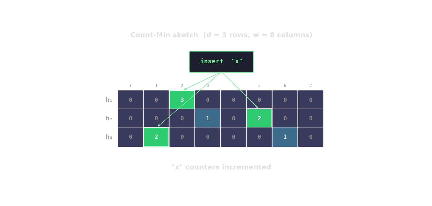
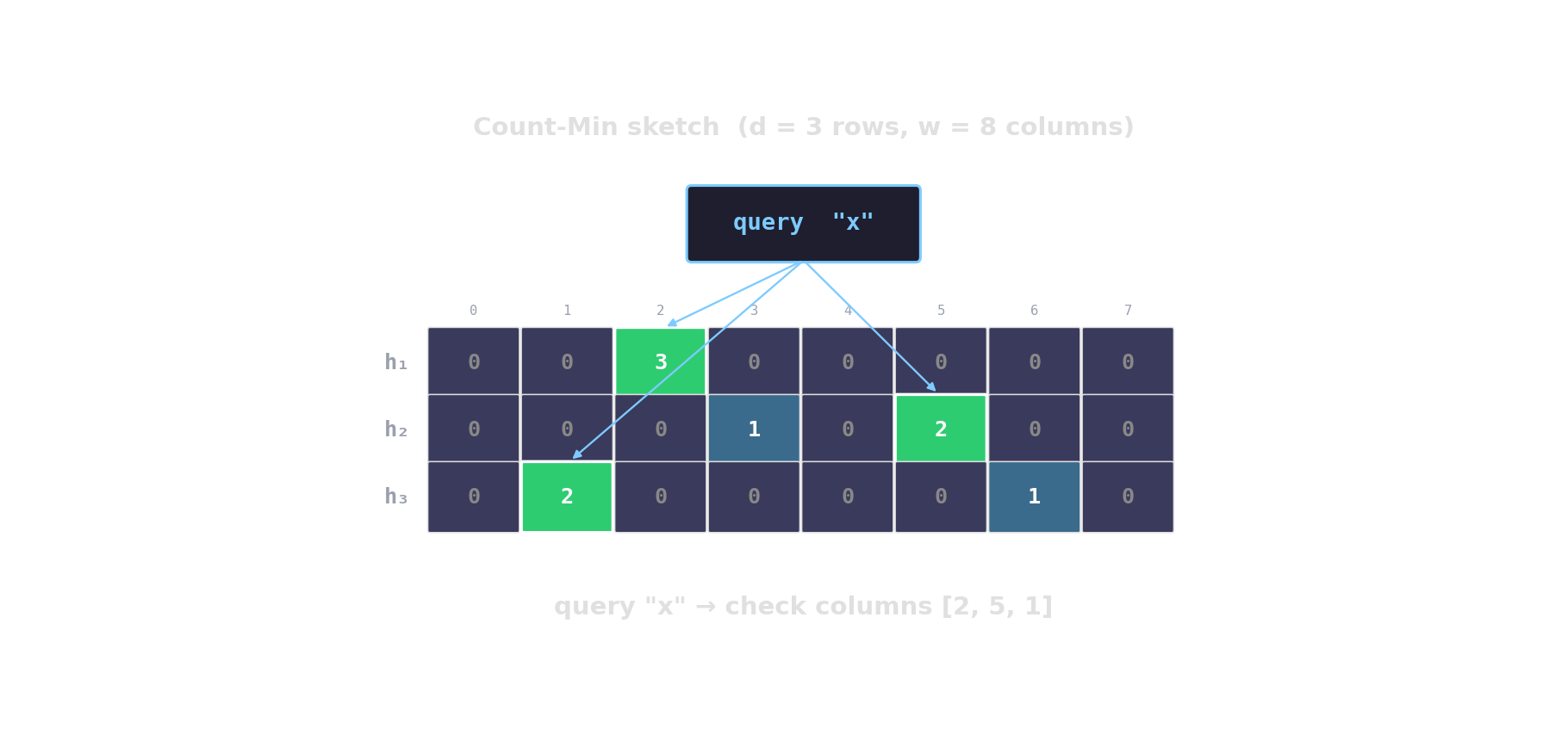
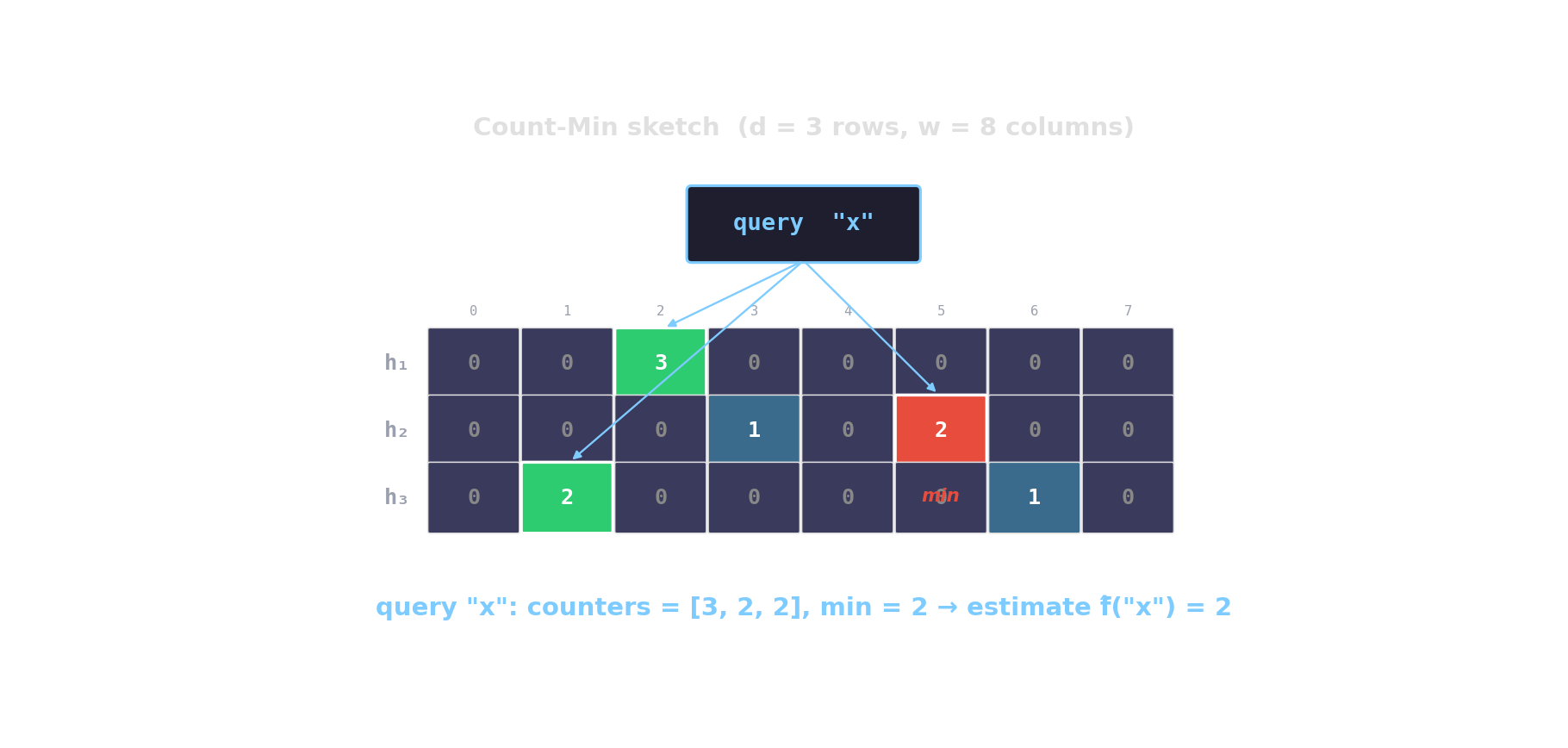
Count-Min sketch — approximate frequencies

d rows, w columns. Hash each item into one cell per row; increment. Query returns the min across rows.

Count-Min — the formal guarantee

\[w = \lceil e/\varepsilon \rceil, \quad d = \lceil \ln(1/\delta) \rceil \;\Rightarrow\; \Pr[\,\widehat{f}(x) - f(x) \le \varepsilon N\,] \ge 1-\delta\]

\(\varepsilon\) controls accuracy (error relative to total stream mass \(N\)).
\(\delta\) controls confidence (probability the bound holds).
Heavy hitters are estimated well; rare items can look noisier in relative terms.

The estimate is always an overcount — never an undercount. The error is bounded by total stream mass, not by the item’s true frequency.

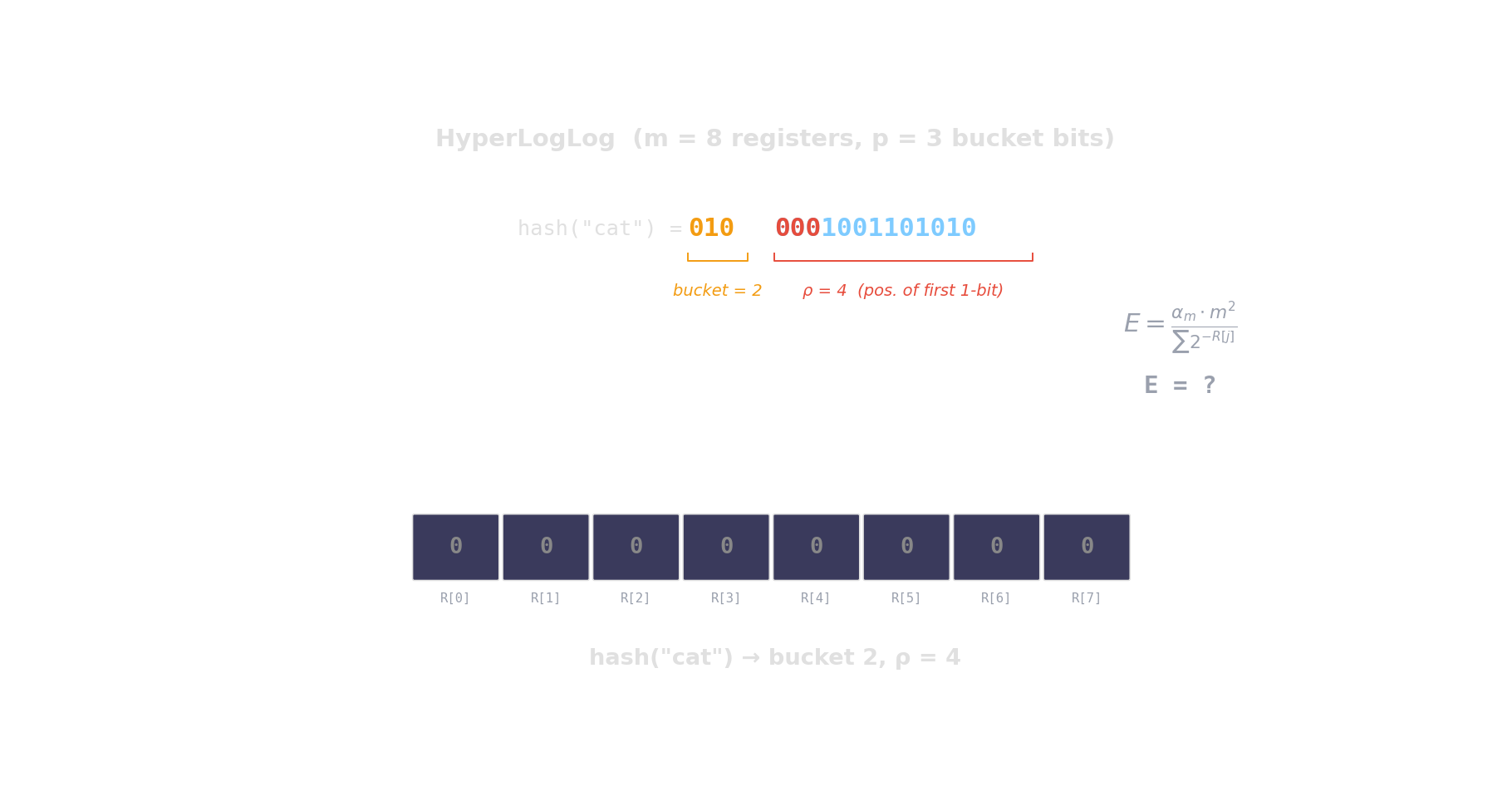
HyperLogLog — distinct-count in kilobytes

Hash each item → count leading zeros → the more distinct items, the higher the maximum.

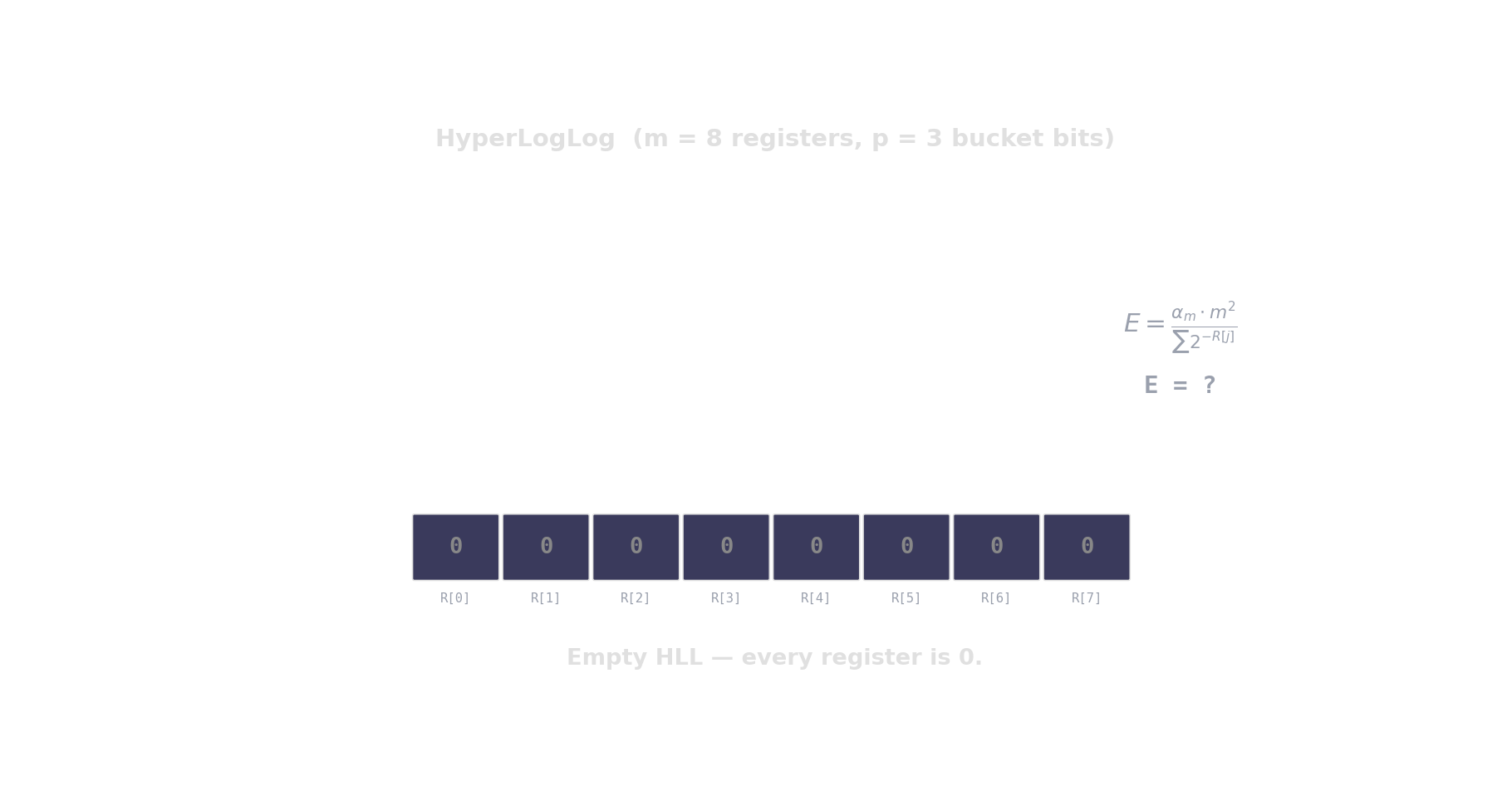
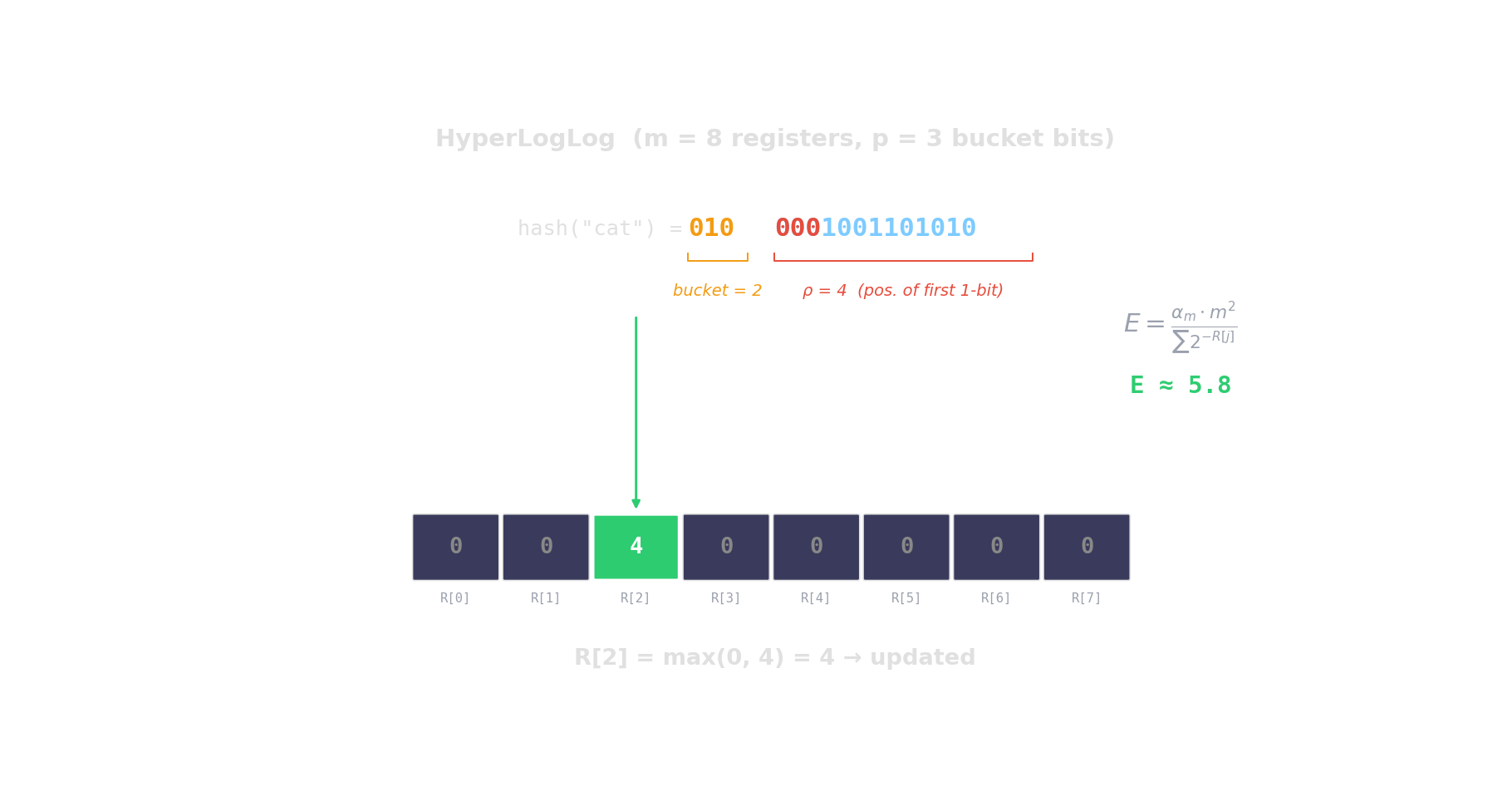
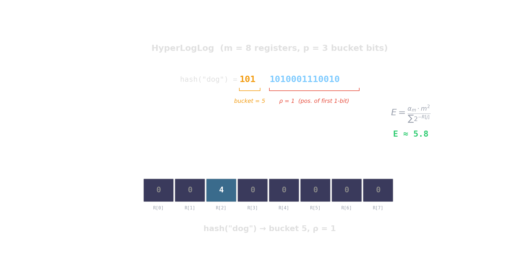
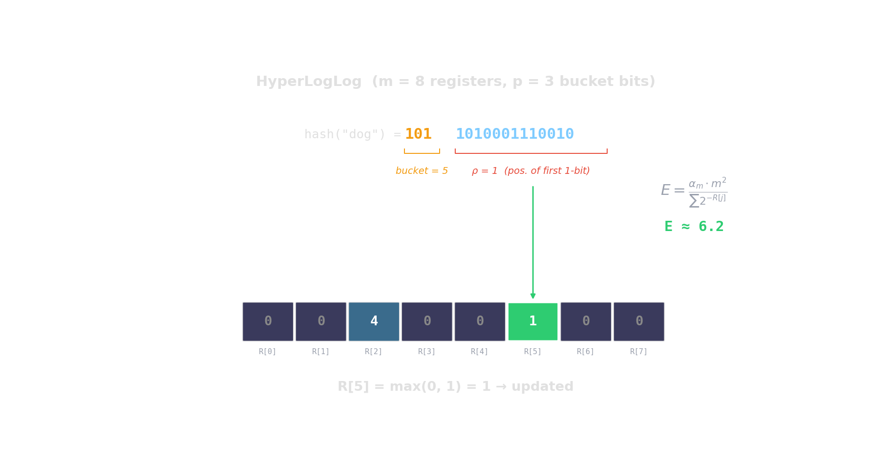
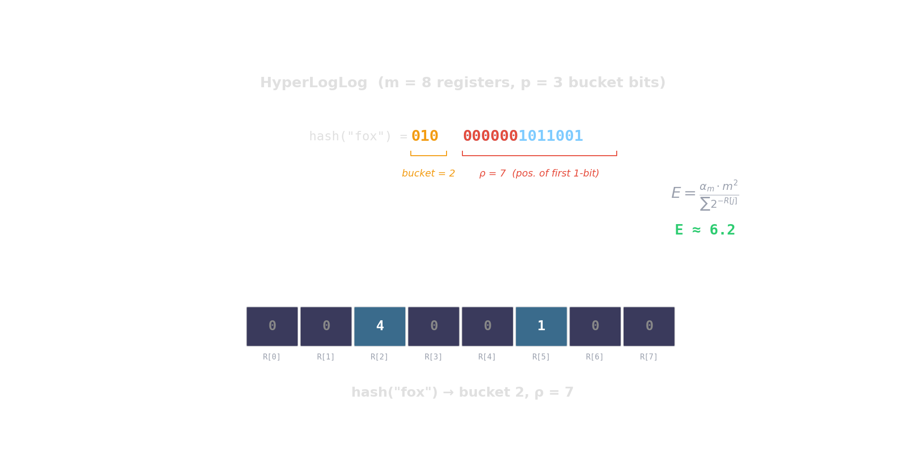
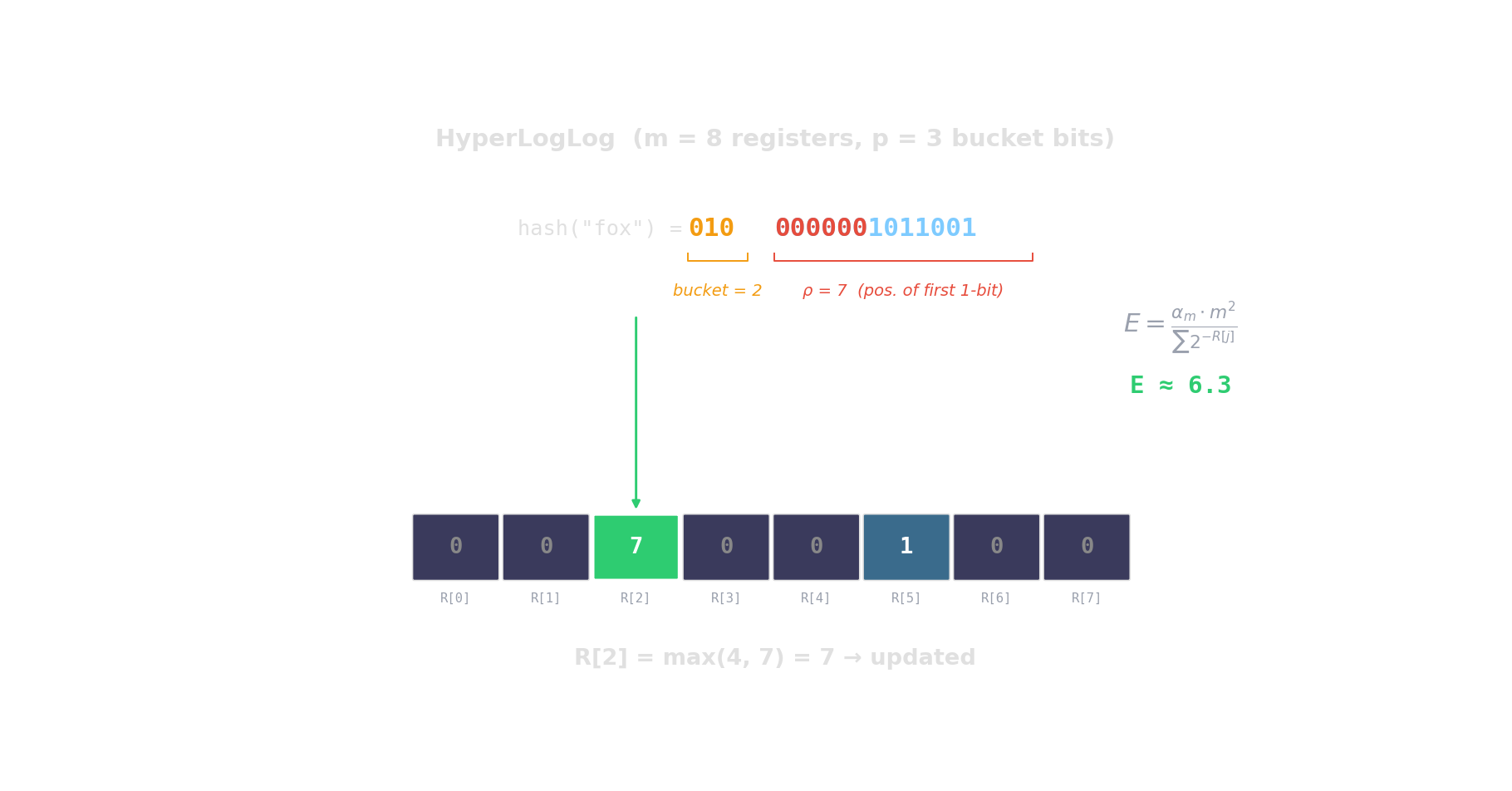
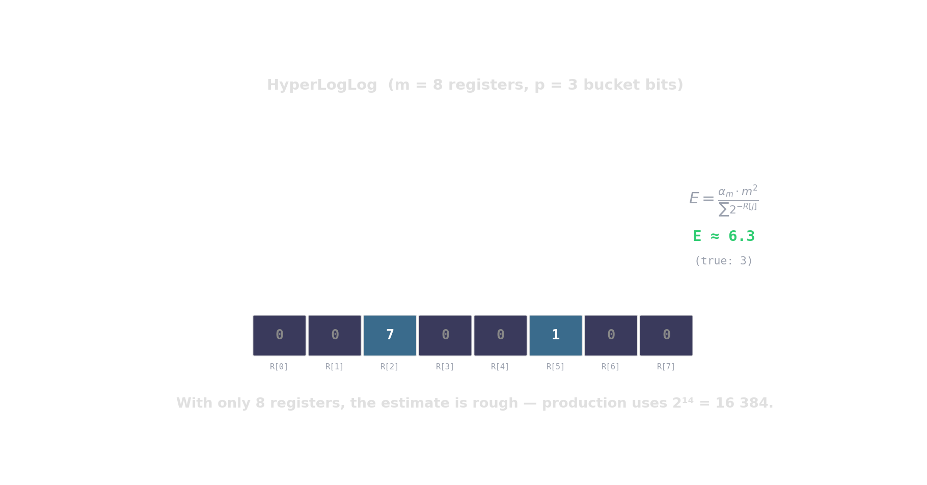
\(2^{14}\) registers = 12 KB \(\Rightarrow\) ~0.8 % error. Redis PFCOUNT, BigQuery APPROX_COUNT_DISTINCT.

Summary — probabilistic structures

	Bloom	Count-Min	HyperLogLog
Question	“seen it?”	“how often?”	“how many distinct?”
Answer	bit vector	min of `d` counters	leading-zero stats
Error	false positives (no FN)	one-sided overcount \(\le \varepsilon N\)	rel. std. err. \(\approx 1.04/\sqrt{m}\)
Classic use	LSM read skip	heavy hitters	`COUNT(DISTINCT …)`

Same recipe, three questions. Reach for them when an exact structure would blow the memory budget — otherwise just use a hash set.

Wrap-up

The data structure is the performance story.

What we covered

Linear

vector first, the rest rarely

Hash maps

open addressing, not chaining

Sorted

B-tree over red-black

Priority queues

implicit tree in an array

Union-find

twenty lines, near-constant

Graphs

CSR: two flat arrays

Spatial

grids, kd-trees, BVH, R-trees

Probabilistic

accuracy for space

What we did not cover

Strings: suffix arrays, suffix trees, tries, FM-index. Their own world.
Persistent / functional: immutable structures, path copying, versioned data.
Concurrent / lock-free: hash maps, queues, trees under contention.
External-memory: real B-trees on disk, LSM trees (RocksDB, LevelDB).
Succinct / compressed: wavelet trees, RRR bit-vectors, rank/select.
More sketches: Cuckoo filter (deletable membership), t-digest (quantiles), MinHash (set similarity).
GPU-oriented: hash tables, BVHs, sort-based primitives on device memory.

Appendix — Reference

For lookup after the lecture. Not covered in the recorded walkthrough.

C++ / Python cheat sheet

Topic	C++	Python
Dynamic array	`std::vector`	`list`, `numpy.ndarray`
Small / inline vector	`absl::InlinedVector`, `boost::small_vector`, `llvm::SmallVector`	— (fall back to `list`)
Deque / FIFO	`std::vector` with read index	`collections.deque`
Hash map (default)	`absl::flat_hash_map`, `ankerl::unordered_dense`, `boost::unordered_flat_map`	`dict` (already flat, open-addressed)
Hash map (std)	`std::unordered_map` — chained, avoid when possible	—
Sorted lookup (static)	sorted `std::vector` + `std::lower_bound`	`bisect` on a sorted `list`
Sorted (mutation-heavy)	`absl::btree_map`, `absl::btree_set`	`sortedcontainers.SortedList` / `SortedDict`
Sorted (std)	`std::map`, `std::set` — red-black tree, avoid	—
Priority queue	`std::priority_queue`, `boost::d_ary_heap`	`heapq` on a `list`
Union-find	20-line inline implementation	`scipy.cluster.hierarchy.DisjointSet`, `networkx.utils.UnionFind`
Graph (CSR)	hand-rolled CSR; GraphBLAS, Galois, Ligra	`scipy.sparse.csgraph`, `igraph`, `rustworkx`
Graph (dict-of-dicts)	— (avoid)	`networkx` — fine below ~10⁵ edges
Spatial (kd-tree, BVH, R-tree)	CGAL, nanoflann, Intel Embree, boost::geometry	`scipy.spatial.KDTree`, `scipy.spatial.cKDTree`, `rtree`
Bloom filter	folly, RocksDB, Abseil	`pybloom-live`, `rbloom`
Count-Min / HyperLogLog	`datasketches` (Apache)	`datasketches`, `probables`

Rule of thumb: in Python, reach for a native-code library (NumPy, SciPy, Abseil-via-pybind11) before a pure-Python container when the workload is the bottleneck. In C++, reach for Abseil/Boost flat containers before the std:: ordered or chained defaults.

See you next time

References

Carpenter, Kevin. 2024. Back to Basics: Almost Always Vector.

Carruth, Chandler. 2014. Efficiency with Algorithms, Performance with Data Structures.

Carruth, Chandler. 2016. High Performance Code 201: Hybrid Data Structures.

Jiang, Danny. 2025. Data Structures in Practice: A Hardware-Aware Approach for System Software Engineers.

Mehlhorn, Kurt, and Peter Sanders. 2008. Algorithms and Data Structures: The Basic Toolbox. Springer.

Wirth, Niklaus. 1976. Algorithms + Data Structures = Programs. Prentice-Hall.

Fundamental Data Structures

Welcome

Linear Structures

The choice decides the layout

What a pointer hop actually costs

When does std::list actually win?

std::deque — the Swiss army knife nobody should open

Prefer vector-as-queue

Small-buffer optimization

Summary — linear structures

Hash Maps

When do we actually reach for a hash map?

std::unordered_map is a linked list in disguise

Open addressing — keep collisions local

Swiss tables — split metadata from data

Tuning: reserve, load factor, hash quality

Summary — hash maps

Sorted Containers

When do we actually need order?

Lead with the simplest thing: sorted std::vector

std::map is a red-black tree

Height is the cost

B-tree: same keys, one cache line per node

Choosing the order: match the cache line

B+ tree: routing on top, values in leaves

Summary — sorted containers

Priority Queues

When do we actually need a priority queue?

Binary heap: implicit tree in a flat array

push: append, then bubble up

pop: swap root with last, then sift down

Height is the cost — widen the tree

Modifying the key? Push a new entry instead

Summary — priority queues

Union-Find

Two operations

Two ideas, near-constant time

Twenty lines

Inverse Ackermann — and why it does not matter

Summary — union-find

Graphs

Why graphs matter

Compressed Sparse Row — two flat arrays

Annotated graphs — where do weights live?

Adjacency matrix — when the graph is dense

Bonus: the matrix is an algorithm

When the graph mutates

Summary — graphs

Spatial Data Structures

When do we need them?

Uniform grid — the boring, often-winning baseline

kd-tree — recursive median splits

BVH — the ray-tracing workhorse

R-tree — rectangles in a database

Delaunay triangulation — geometry → sparse graph

Summary — spatial structures

Probabilistic Structures

Bloom filter in action

Where does the false-positive rate come from?

Sizing a Bloom filter in practice

Count-Min sketch — approximate frequencies

Count-Min — the formal guarantee

HyperLogLog — distinct-count in kilobytes

Summary — probabilistic structures

Wrap-up

What we covered

What we did not cover

Further reading

Appendix — Reference

C++ / Python cheat sheet

See you next time

References

When does `std::list` actually win?

`std::deque` — the Swiss army knife nobody should open

`std::unordered_map` is a linked list in disguise

Lead with the simplest thing: sorted `std::vector`

`std::map` is a red-black tree