Graph & Network Algorithms

Algorithm Engineering — L08

Dr. Dominik Krupke

Welcome

Graphs: a quick recap

Graph vocabulary used in this lecture.

Anatomy of a graph

• Nodes: any kind of entities, like people, places, tasks, states.
• Edges: relationships between pairs of nodes, like connections, precedence, transitions.
• Weights and data: edges (and nodes) carry numbers, time, cost, capacity.
• Direction: an edge may be one-way.

Cycle-free graphs

DAG (Directed Acyclic Graph):

Tree:

The topological structure of cycle-free graphs often allows efficient handling via dynamic programming, even for cases that would be hard on general graphs.

Common Graph Problems

“A wise platypus will solve a graph problem with a graph algorithm, for LPs are more general, but graph algorithms are faster.”

— Confucypus

Shortest Paths

A minimum-weight path from a source to a target in a weighted graph.

Definition: the shortest-path problem

A weighted graph \(G = (V, E)\) with edge weights \(w(u,v)\), a source \(s\), a target \(t\).

A path is a sequence of edges \[s = v_0 \to v_1 \to \dots \to v_k = t,\] and its length is \(\sum_i w(v_{i-1}, v_i)\).

The shortest path is one of minimum total length.

Not just routing

• Routing is the most popular and most visible shortest-path application.
• Intersections are nodes, roads are edges, and each weight is travel time.
• From source to target, the minimum-weight path is the fastest route.
• The same idea appears beyond maps:
  • Cheapest transition sequences in state spaces.
  • Best schedules in roster grids.

Rostering: which shifts are hard to staff?

Some shifts are harder to fill than others.

• Assign workers one by one, prioritizing hard-to-cover shifts.
• Incompatible shifts make the best coverage non-trivial.
• For one worker, the best schedule is a shortest path on a DAG.

In practice, this works very well with advanced pricing and column generation.

Shift generation as a DAG shortest path

Per worker, create a DAG with the allowed transitions and the weights of the slots.

Negative weights to reward hard-to-fill slots.

The SP represents the best schedule for that worker, given the remaining demand.

DAG allows a linear DP here!

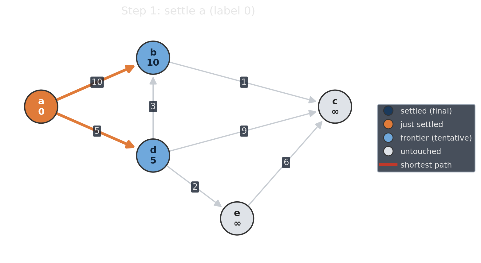
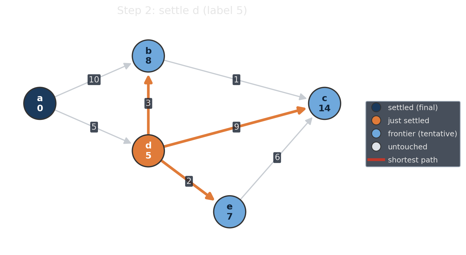
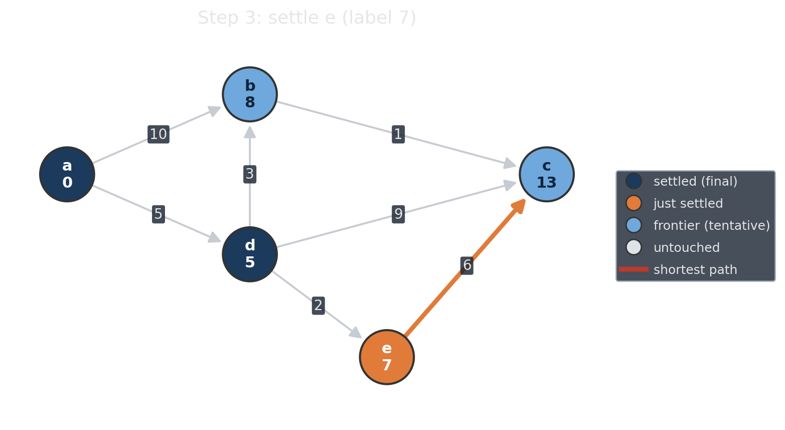
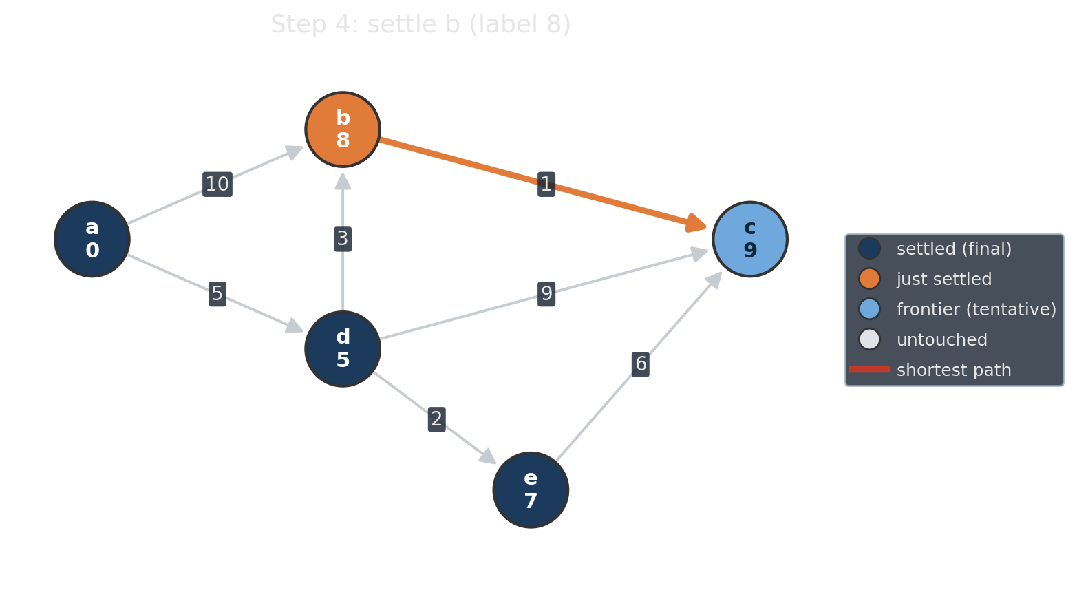
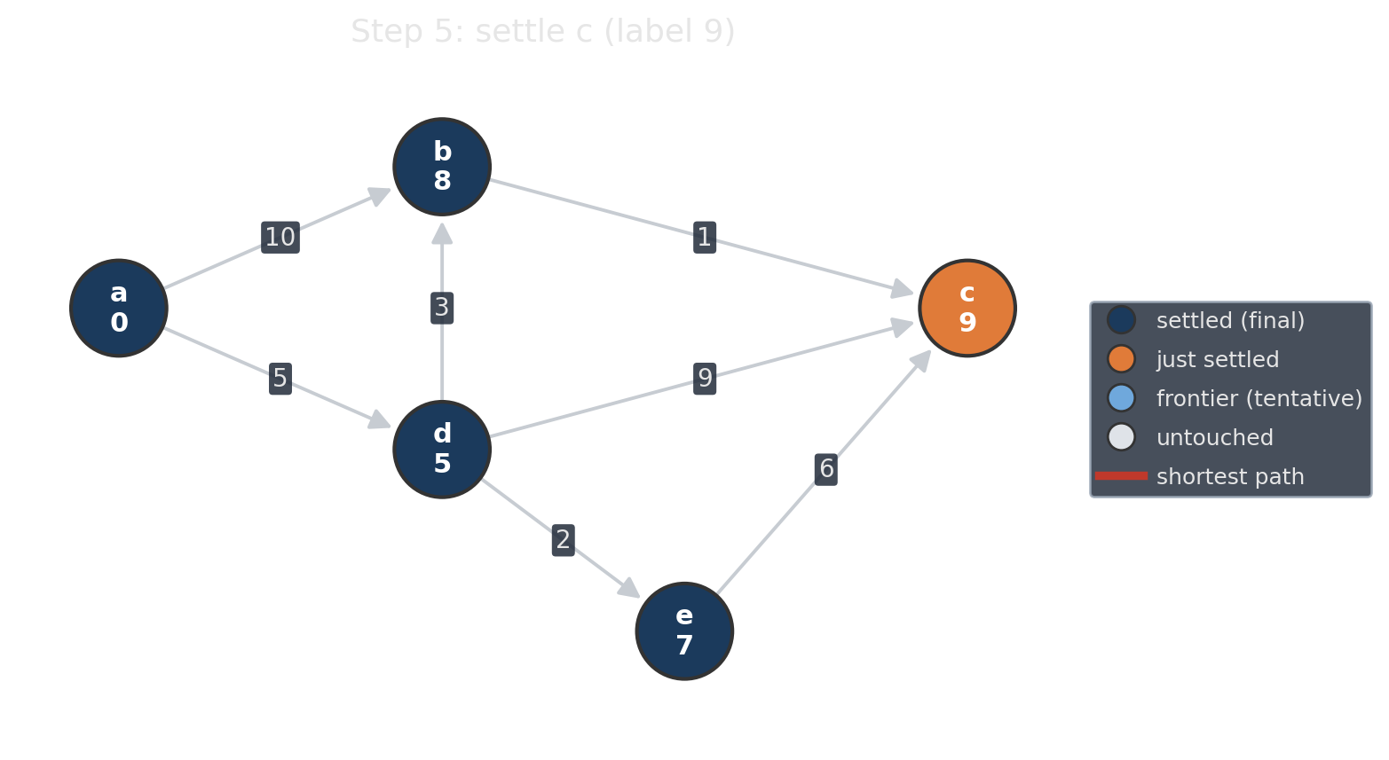
Dijkstra: label-setting, step by step

Keep a tentative distance on every node.

1. Settle the frontier node with the smallest tentative label. Its label is now final.
2. Relax its out-edges: improve neighbors’ labels.
3. Repeat until the target settles.

A*: Adding information to guide the search

Tiny change to Dijkstra: add a heuristic underestimation of the remaining cost to the target.

\[f(v) = \underbrace{g(v)}_{\text{cost so far}} + \underbrace{h(v)}_{\text{estimate to } t}.\]

• Admissible (\(h\) never overestimates) keeps A* optimal.
• Consistent (\(h(u) \le w(u,v) + h(v)\)) settles each node once, just like Dijkstra.

Dijkstra is A* with \(h \equiv 0\).

nx.astar_path(G, s, t, heuristic=h, weight="weight")

Dijkstra vs. A*: flood vs. cone

Choosing a Shortest-Path Algorithm

Query model

• One \(s \to t\): Dijkstra with early stop; A*
• One \(s \to V\): Dijkstra / Bellman-Ford
• All pairs: Floyd-Warshall / Johnson
• Many queries: preprocessing-based methods

Graph assumptions

• Unweighted: BFS
• Nonnegative weights: Dijkstra
• Negative weights: Bellman-Ford
• DAG / layered graph: dynamic programming
• Dense APSP: Floyd-Warshall
• Sparse APSP: Johnson

Engineering questions

• Can we stop early?
• Is there a useful admissible heuristic?
• Is preprocessing worth the memory and setup time?

Time-dependent shortest paths

With time-dependent costs, how long an arc takes depends on when you enter it (rush hour).

FIFO (“no overtaking”): arrival time is non-decreasing in departure time. Leaving later never lets you arrive earlier. Then the optimality principle holds and Dijkstra is unchanged: evaluate travel time at the current arrival time.

Using A* to search solution spaces

Dijkstra and A* need only two things: a successor function and a frontier, not the whole graph.

This sliding puzzle has ~180,000 states. A* only touched 283 by having a heuristic that lower bounds the distance to the solution.

Same structure as branch-and-bound, planning, motion planning: a graph you generate, never store. The heuristic aims at the goal configuration but is usually inexact.

Resource-Constrained Shortest Path

Time-dependent costs look hard but are easy, negative edges and resource constraints look easy but are hard.

A very common subproblem in optimization is to find a cheapest path that respects a resource limit. That is the Resource-Constrained Shortest Path, and it is NP-hard.

Weakly NP-hard with one integer resource; strongly NP-hard with several.

Matching

A matching is a set of edges, no two sharing a vertex. Bipartite graphs admit a clean linear program; an odd cycle makes the problem harder.

Definition: matching, maximum, and weighted

A matching \(M \subseteq E\): no two edges share a vertex.

• Max-Cardinality, min-weight: find the largest matching of minimum total weight.
• Max-weight: weights \(w_e\); maximize \(\sum_{e \in M} w_e\).
  • Not necessarily cardinality-maximal: a smaller matching can have higher weight.

Two special cases:

1. Integral weights tend to be more robust than fractional ones.
2. Bipartite graphs allow faster algorithms.

Example: Kidney exchange

Match compatible pairs of donors and patients, where the willing donor is not compatible to their own beneficiary. Maximize expected number of successful transplants.

See also the AlgLab exercise of a more complicated version: https://github.com/d-krupke/AlgLab-WS2526-material/tree/main/sheets/01_cpsat/exercises/03_organ_donor_problem

Weighted matching = the assignment problem

Edges carry costs. Five orders, five machines: each order runs on one machine, each machine takes one order. Minimize total cost. That is a minimum-cost perfect bipartite matching.

Flows

Pushing units through a capacitated network from a source to a sink.

Flow Problems: From Throughput to Cost

Max flow

A capacitated network with source \(s\) and sink \(t\).

Goal: send as much flow as possible from \(s\) to \(t\).

Min-cost flow

A network with supplies/demands, capacities, and per-unit edge costs.

Goal: satisfy all balances at minimum total cost.

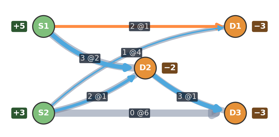
Same modeling primitive, different objective:
move flow subject to conservation and capacities.

Min-cost flow subsumes shortest path, assignment, transportation, and fixed-value flow problems.

A logistics problem: redistributing empty crates

A logistics company runs trucks between four depots (A, B, C, D) every day. Goods travel in reusable crates, and the empties piggy-back on regular deliveries — but each truck only has a few empty-crate slots per trip.

Demand is asymmetric, so over a few days some depots accumulate surpluses of empties while others run short and start delaying outbound deliveries.

Question. Given the surplus / shortage pattern and the truck slot capacities, how many crates can we redistribute in time to reduce the shortages — and what is the bottleneck?

Modelling it as max flow on a time-expanded graph

Min-cost flow: a schedule as a flow

Six tasks, fixed times, each at a station. Moving between stations costs a 30-minute changeover. Cover every task at minimum wage.

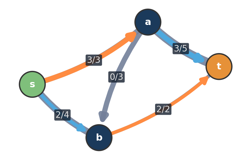
The residual graph

Flow on the network

Residual graph (find a path, push, repeat)

Step 3’s only path runs backward along \(c \to a\): it cancels flow pushed in step 1. A forward-only construction has no such arc; residuals provide it.

When flows get complicated

Single-commodity flow is polynomial and integral. Variants push past that polytope:

• Multi-commodity (several goods sharing capacities): fractional optimum, integer version NP-hard.
• Fixed/activation costs (pay to open an edge or facility): no longer a pure flow.
• Side constraints (e.g., a resource budget).

The flow backbone usually survives. The polytope stays near-integral, so a MIP solver branches only on the few messy variables. Model the flow part as a flow; the solver handles the rest.

Spanning Trees

The minimum-weight set of edges that connects every vertex of a weighted graph.

Definition: spanning tree, and the minimum spanning tree

A spanning tree of a connected graph: a subset of edges that touches every vertex and has no cycle. Always exactly \(n - 1\) edges.

The minimum spanning tree (MST) is the spanning tree of least total weight.

Kruskal, Prim, Borůvka: three greedy strategies, all reaching the same optimum. For the MST, greedy is provably exact.

Wiring a campus: cheapest fiber backbone

Every building needs a high-speed link to the central data center. Connect every building with the least total trench length.

Summary

Cheapest transitions.

Pairing/Assignment.

Balanced Production/Circulation/Consumption.

Cheapest Skeleton/Network.

While matching and flow algorithms often scale well in practice, they have a roughly cubic worst-case complexity, which for certain instances can become critical.

Course Evaluation

Please take 10–15 minutes to fill out the survey.

https://umfragen.tu-bs.de/evasys/online.php?pswd=9728N

• Evaluation week: 01.–07.06.2026
• Anonymous, via EvaSys

See you next lecture