Beyond the Single Objective: Trade-offs and Uncertainty

Algorithm Engineering — L13

Dr. Dominik Krupke

Welcome

Beyond \(\min f(x)\)

One objective, trusted data. Real systems rarely grant either.

What is missing from the standard optimization model?

The textbook model has a clear objective and static data: \[ \min \{ f(x) \mid x\in\mathcal X \} \] Frequently, we do not have this in practice.
Quality is multidimensional. Tardiness, changeovers, plan stability: improving one can worsen another. What does better mean?

Reality is uncertain. Forecasts are wrong, measurements are stale, and execution deviates from plan. What world will we face?

Part I: Multiple Objectives

Improving one objective can worsen another. Which solution is better?

Three repairs for a broken plan

A machine failed overnight. The production schedule must be rebuilt, and three repairs are feasible:

repair total tardiness changeovers changed jobs
A 100 min 20 35
B 120 min 12 30
C 150 min 25 40

All three columns matter: late orders pay penalties, changeovers consume capacity, and every changed job disrupts the shop floor.

Which repair is best?

C loses to both A and B in every column. A versus B is a genuine trade-off: the objective values alone do not tell us which is better.

Dominance and the Pareto front

For minimization, \(x\) dominates \(y\) iff

\[ \forall i: f_i(x)\le f_i(y), \; \exists j:f_j(x)<f_j(y). \]

Dominated solutions are unambiguously inferior (within the modeled objectives).

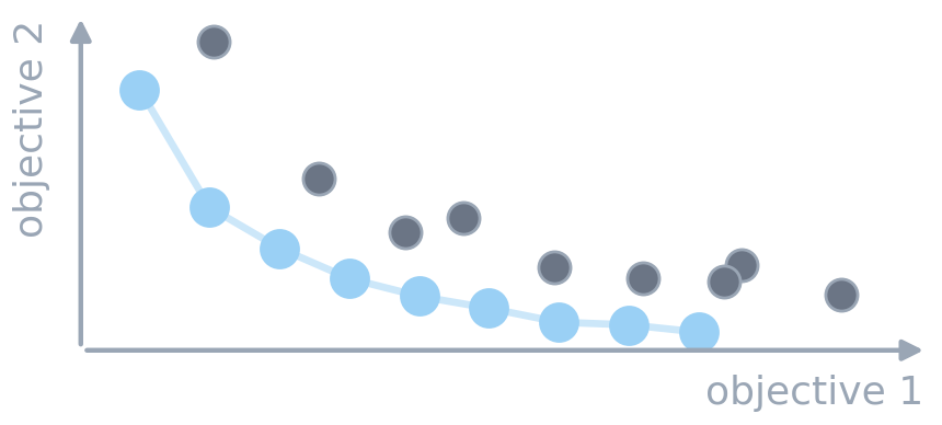
For visualization, consider only tardiness and changeovers. Their nondominated objective vectors form the shown Pareto front.
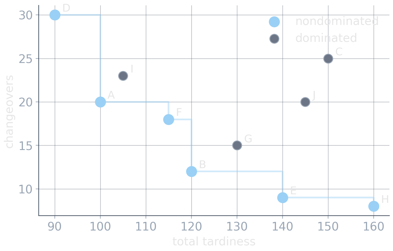
Pareto-optimal does not mean good. A terrible-but-nondominated solution is still terrible. And the front is a concept, not an algorithm.

Preference model vs. search method

Preference / decision model

How do objective vectors become a decision?

  • weighted sum
  • lexicographic order
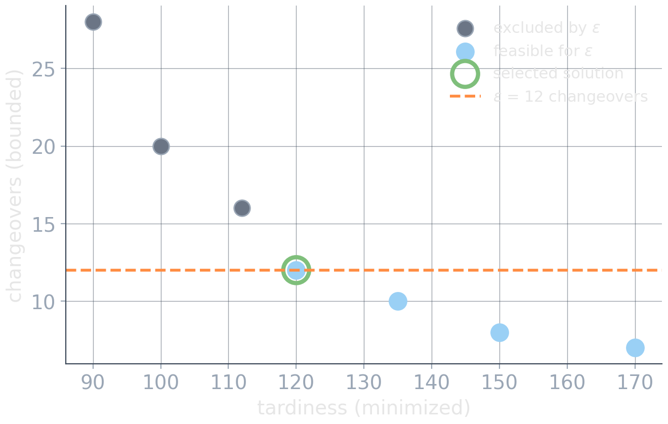
  • \(\epsilon\)-constraints
  • a human picks from the front
  • feedback loops, learning, or other adaptation

Search method

How are good solutions found?

  • exact solvers: MIP, CP-SAT
  • ILS, LNS, VNS, R&R, beam search
  • population-based search

Keep the questions separate: how do we compare solutions? and how do we find them? Many combinations are possible.

One Solution: Encode the Preferences

If someone can say what better means, write it into the model. The methods differ in what they ask that someone to know.

Weighted combination

\[ \min_x\; \sum_i w_i\, f_i(x) \quad\leadsto\quad \min_x\;\; 1.0\cdot\text{tardiness} + 5.0\cdot\text{changeovers} + 0.2\cdot\text{changed jobs} \]

Strengths

  • reuse single-objective machinery
  • one actionable answer
  • simple to set up

Fine print

  • units matter silently: minutes vs. counts
  • linear compensation: enough gain elsewhere can justify any loss
  • where do the \(w_i\) come from?

The weights act as exchange rates. This model declares one changeover worth exactly five minutes of tardiness. Who signed off on that?

Two traps of the weighted sum

Trap 1: scale. Normalizing to reference ranges

\[ \tilde f_i(x) = \frac{f_i(x)-r_i^{\text{low}}} {r_i^{\text{high}}-r_i^{\text{low}}} \]

fixes units, not preferences. The reference ranges are themselves modeling choices, and changing them changes the answer.

You also do not always know what sensible ranges are if this is based on customer data.

Trap 2: reachability.
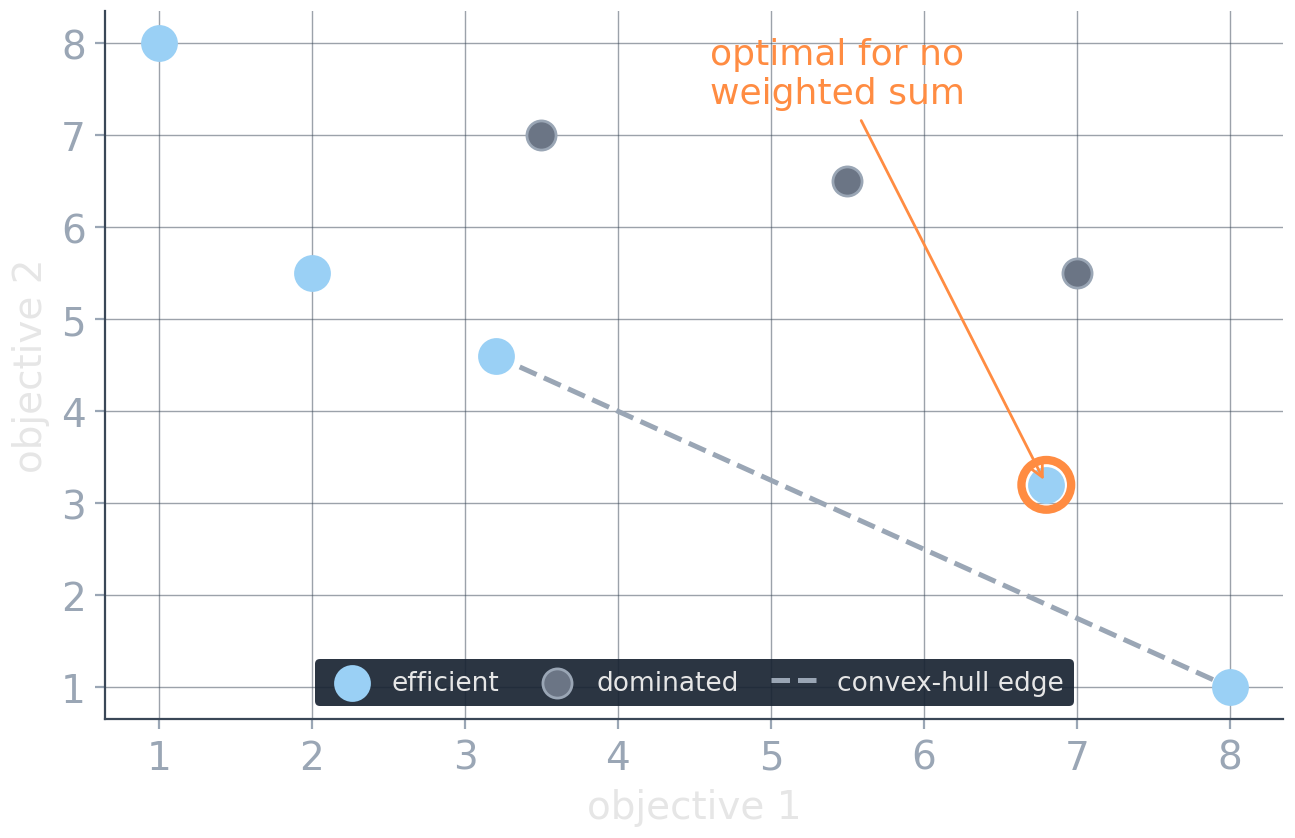
In discrete problems, some efficient solutions are optimal for no nonnegative weight vector. Sweeping weights will never show them to you.

Lexicographic optimization

\[ \operatorname{lexmin}\big(f_1(x),\, f_2(x),\, \dots,\, f_k(x)\big) \]

Implemented as sequential solves, each preserving the optimum of the previous level:

\[ z_1^* = \min f_1(x) \]

\[ z_2^* = \min\{\,f_2(x): f_1(x)=z_1^*\,\}, \;\;\dots \]

Or allow a deliberate slack before optimizing the next level:

\[ f_1(x)\le z_1^*+\Delta \quad\text{or}\quad f_1(x)\le(1+\delta)z_1^*. \]

candidate rejected tardiness changeovers
A 0 400 min 3
B 1 0 min 0

With rejected orders as first priority, A wins, however ugly the rest: higher levels have infinite precedence.

Tricks like \(\min\, M f_1 + f_2\) are dangerous.

Many solvers have inbuilt support for lexicographic objectives, including slack.

Bounds instead of weights: \(\epsilon\)-constraints

\[ \begin{aligned} \min_x\quad & f_1(x)\\ \text{s.t.}\quad & f_2(x)\le \epsilon_2\\ & f_3(x)\le \epsilon_3 \end{aligned} \]

How requirements are often stated:

  • service level at least 95%
  • at most 20 plan changes
  • emissions below the permit

You can also combine this with other methods, or making this soft-constraints, maximize the number of satisfied bounds, etc.

Many Solutions: Expose the Trade-off

When nobody can name the exchange rate, do not guess it. Compute the alternatives.

Produce alternatives, then decide

Preferences are often formed by seeing trade-offs, not before.

Worth computing:

  • the extremes: best of each single objective
  • balanced compromises in between
  • knee regions: favorable local trade-offs
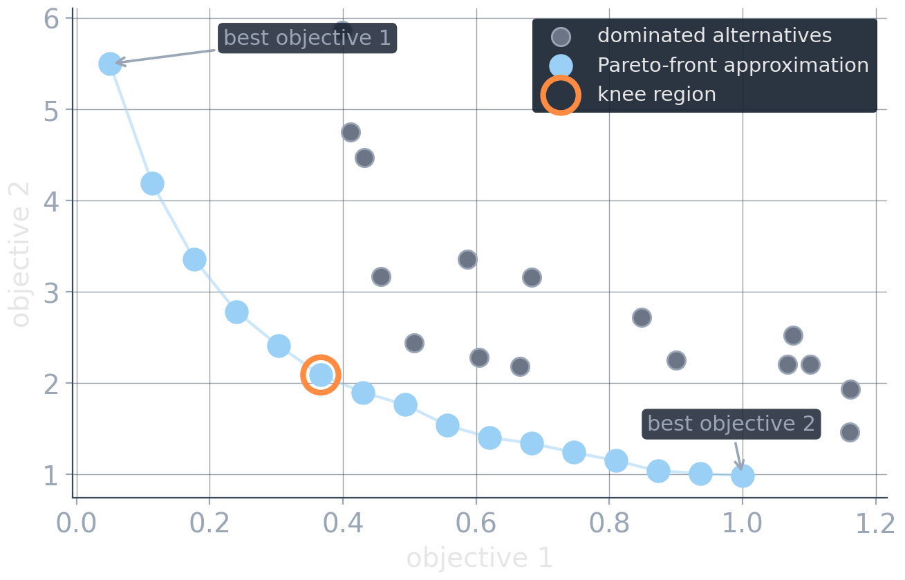
The output of optimization becomes a set. The decision happens afterwards, with a human in the loop.

A controller around the solver you already have

for setting in preference_grid:          # a weight λ or a bound ε
    solve the single-objective problem   # reuse state / warm-start when helpful
    add candidate(s) to archive, dropping dominated entries

Weighted sweep: vary \(\lambda\) in \(\min_x\; \lambda f_1(x) + (1-\lambda) f_2(x)\)

  • simple controller reusing the existing solver
  • blind to unsupported points

\(\epsilon\)-sweep: vary \(\epsilon\) in \(\min_x\; f_1(x) \;\;\text{s.t.}\;\; f_2(x)\le\epsilon\)

  • recovers unsupported points the weighted sweep misses
  • exact enumeration needs additional conditions

Multi-objective optimization can be a loop around the single-objective solver you already trust.

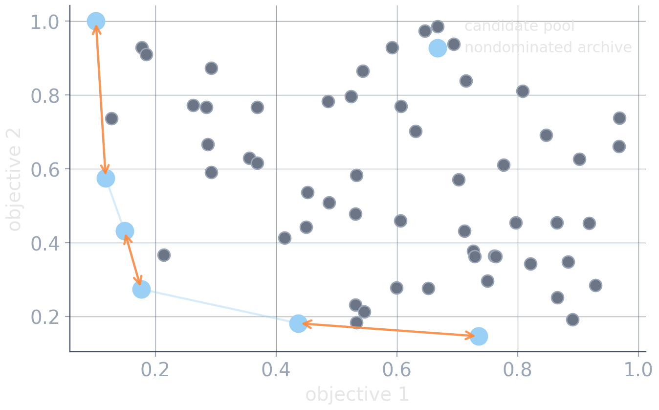
Nondominated archives: keep the trade-offs found so far

For every new candidate \(x\):

  1. discard \(x\) if dominated
  2. otherwise insert \(x\)
  3. remove archive entries dominated by \(x\)

If the archive becomes too large:

  • prune crowded regions
  • preserve coverage of objective space
  • preserve decision-space diversity

An archive is nondominated only relative to the candidates seen so far. Heuristic search does not certify the true Pareto front.

NSGA-II: a canonical population-based example

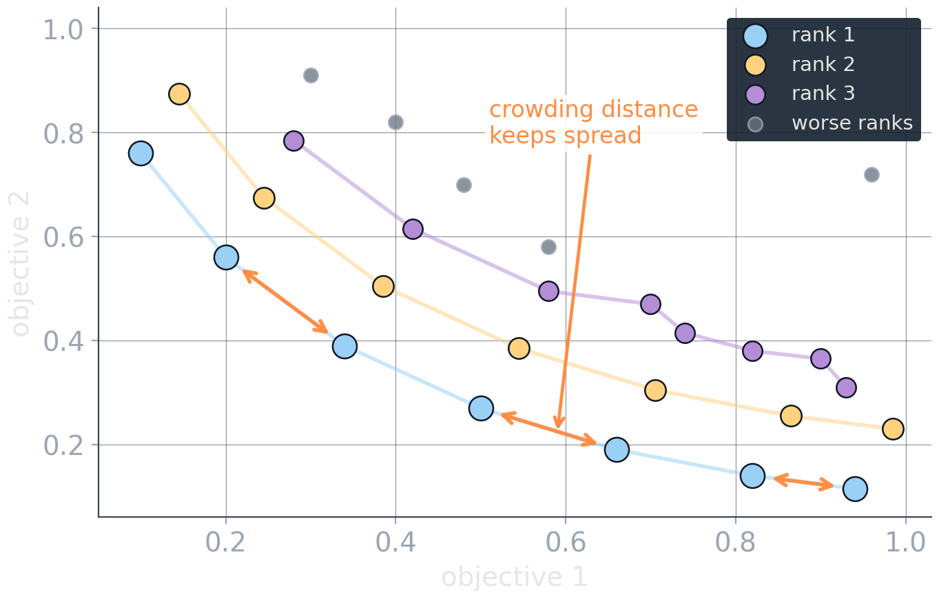
Population selection uses two pressures

  1. quality

    • sort candidates into nondom. fronts
    • prefer better fronts
  2. diversity

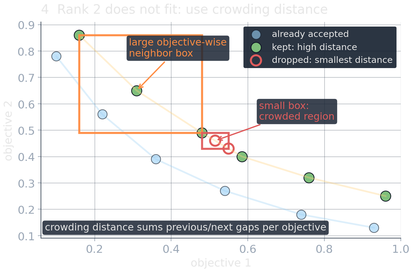
    • use crowding distance within a front
    • avoid filling one narrow region

NSGA-II (Deb et al. 2002) combines these ideas with elitist genetic search.

A genetic algorithm is not automatically the right multi-objective method. If you already have strong problem-specific search, add an archive before replacing it with a generic GA.

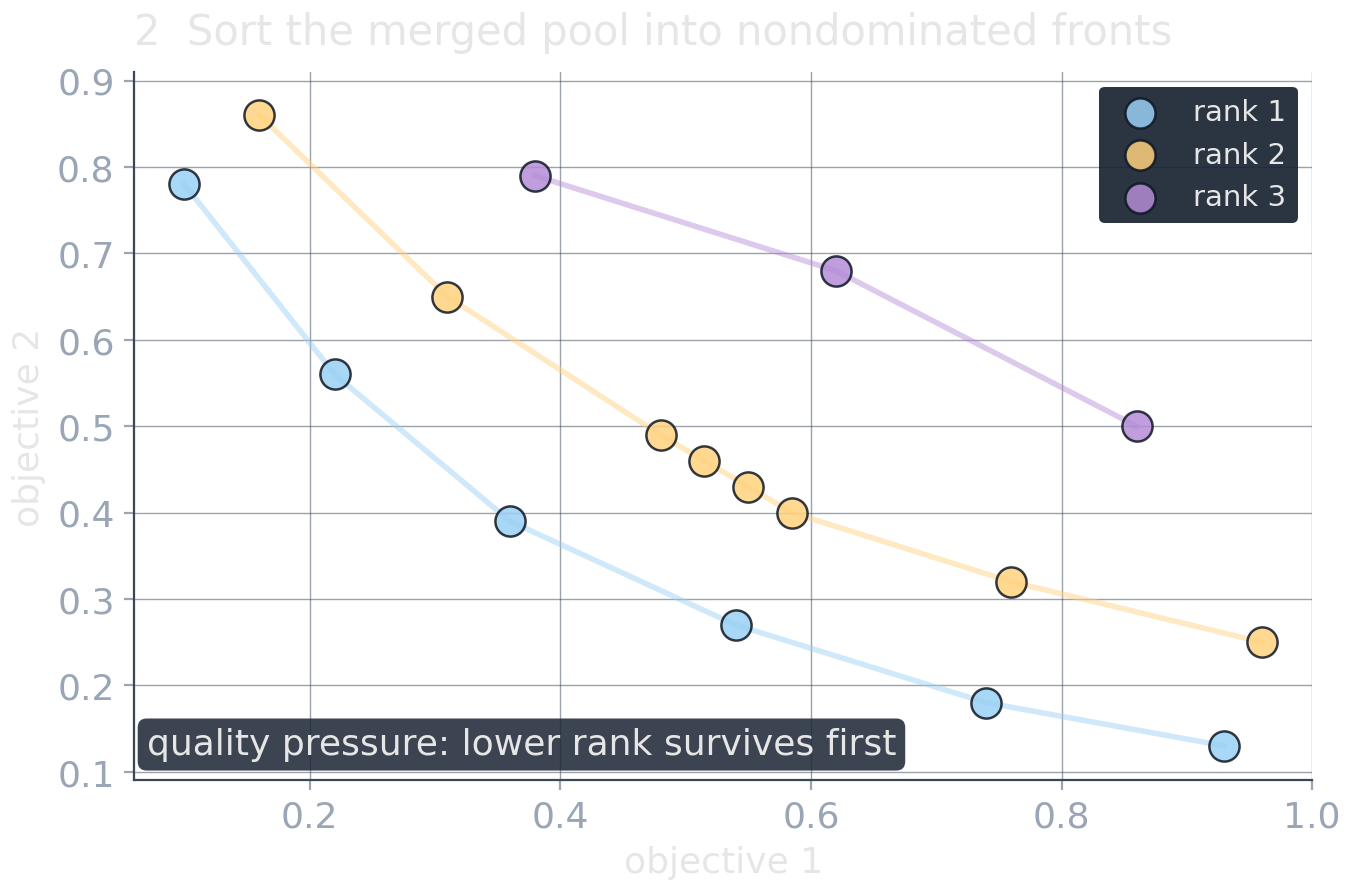
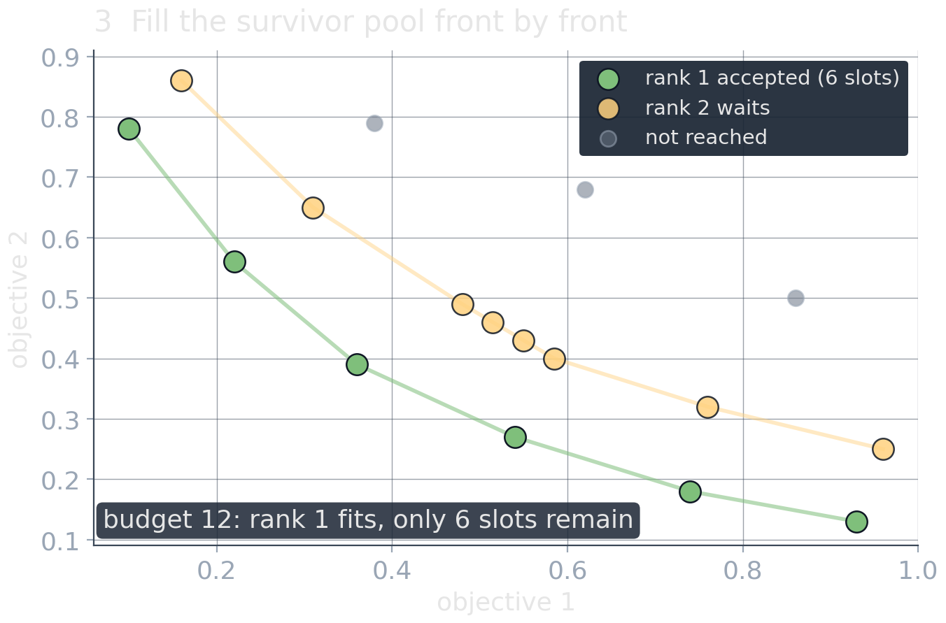
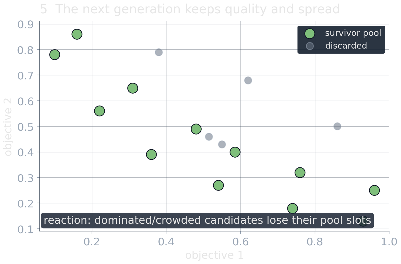
NSGA-II selection: what actually changes?

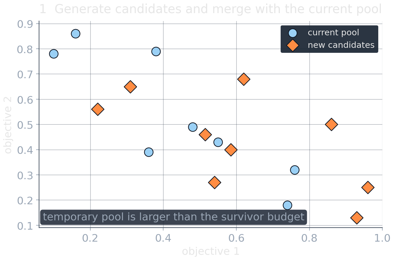
Each generation shrinks a temporary pool back to fixed size.

  1. merge old pool + new candidates
  2. sort into nondominated fronts
  3. accept fronts while they fit
  4. if a front overflows: keep points with largest crowding distance

Crowding distance = objective-wise neighbor boxes.
Choosing a multi-objective strategy

You have… Reasonable first choice
meaningful exchange rates weighted aggregation
a genuinely strict hierarchy lexicographic optimization via sequential solves
strong priorities with some slack sequential solves with additive or meaningful relative tolerance
known hard limits \(\epsilon\)-constraints
unresolved preferences curated nondominated alternatives
a strong single-objective solver weighted or \(\epsilon\) sweeps around it
a strong heuristic search a nondominated archive around it

Part II: The World Is Uncertain

Part I asked what we want. Now: what world will we face?

The newsvendor: one decision, one uncertain number

A bakery decides at 5 a.m. how many sandwiches to prepare. Demand \(D\) reveals itself at lunch.

\(p\) selling price 10 €
\(c\) production cost 4 €
\(v\) evening salvage 1 €

One sandwich short loses the margin

\[ C_u = p-c = 6. \]

One sandwich left over loses

\[ C_o = c-v = 3. \]

Expected demand is 100. Prepare 100?
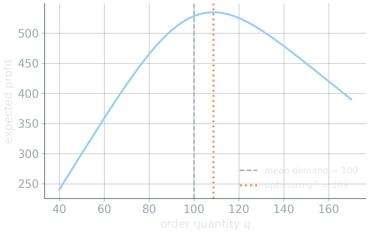
Not a skewed forecast. Demand here is symmetric; the asymmetric costs (\(C_u\neq C_o\)) shift the optimum.

The marginal unit picks a quantile

Prepare one more unit?

For a current quantity \(q\), the marginal unit sells only if demand exceeds \(q\):

\[ \underbrace{C_u\,\mathbb P(D>q)}_{\text{expected gain}} - \underbrace{C_o\,\mathbb P(D\le q)}_{\text{expected waste}} \]
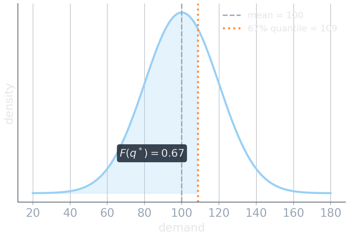
Add units while this is positive:

\[ C_u\big(1-F(q)\big) > C_o\,F(q) \;\;\Longleftrightarrow\;\; F(q) < \frac{C_u}{C_u+C_o} \;\;\Longrightarrow\;\; q^* = F^{-1}\!\left( \frac{C_u}{C_u+C_o} \right). \]

Here: \(\;\alpha=\dfrac{6}{6+3}=\dfrac23\), and with \(D\sim\mathcal N(100,20^2)\): \(\;q^*\approx109\).

The danger of point forecasts

Practice often separates prediction from optimization: predict-then-optimize (PtO).

\[ \begin{aligned} \text{data} &\;\longrightarrow\; \text{prediction } \hat d(x) \\ &\;\longrightarrow\; \text{optimization} \;\longrightarrow\; \text{decision} \end{aligned} \]

Squared-error loss targets the conditional mean \(\mathbb E[D\mid X=x]\); the newsvendor decision needs the conditional quantile \(F^{-1}_{D\mid X=x}(\alpha)\).
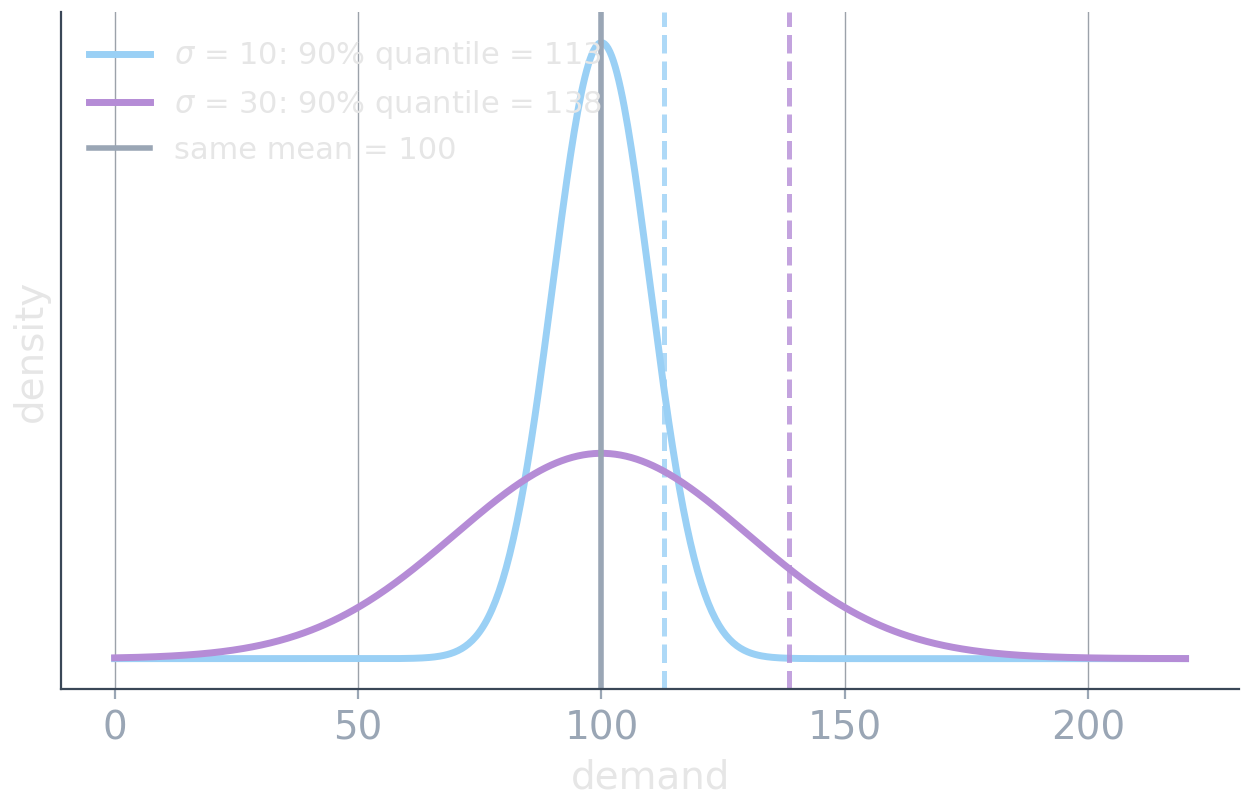
\[ \boxed{ \text{prediction-loss optimal} \;\not\Rightarrow\; \text{decision optimal} } \]

Even a perfect point forecast can be the wrong interface: it discards exactly the uncertainty information the decision needs.

Diagnose Before You Model

“There is uncertainty” is not yet a diagnosis.

Where does the mismatch enter?

mechanism the mismatch typical intervention
forecast / future realization tomorrow’s demand is not yet known better prediction where possible; quantiles, distributions, scenarios
measurement / state current work-in-progress is observed imperfectly sensing, reconciliation, state estimation
parameter model form accepted, coefficient uncertain calibration, sensitivity analysis, uncertainty sets, scenarios
model abstraction omits relevant mechanisms validation, richer model, redesign
execution planned 08:00, actually started 08:17 buffers, feedback, rescheduling, simpler plans

When does the information arrive?

Observe, then decide

\[ \xi \;\to\; x(\xi) \]

For this uncertainty, condition on the observation and optimize.

Decide, then observe

\[ x \;\to\; \xi \]

Here-and-now commitment before uncertainty resolves.

Decide, observe, react

\[ x_1 \;\to\; \xi \;\to\; x_2(\xi) \]

Partial commitment with recourse.

The information structure determines which decisions may adapt: a property of the process, not of the solver.

Rolling horizon: adapt repeatedly

\[ \text{observe} \;\to\; \text{optimize} \;\to\; \text{execute the first steps} \;\to\; \text{observe again} \;\to\; \text{reoptimize} \]

Rolling-horizon reoptimization: defer commitment · incorporate fresh information · absorb disturbances · repeatedly repair the plan

Better feedback and shorter commitment horizons can beat greater conservatism. Not every uncertain problem needs one giant uncertainty-aware model.

Reoptimization is not free: too much replanning can create instability, churn, and plans that nobody trusts.

Three questions before choosing a method

  1. What is uncertain? forecast, state, parameter, model, execution?

  2. What do we know about it? point estimate · bounds · samples · scenarios · probability distribution

  3. When is it revealed, and what can still adapt? before commitment · after commitment · between decision stages · repeatedly over time

Robust Optimization

A set of plausible worlds, and protection against every one inside it.

From one estimate to a set

Nominal planning trusts one estimate:

\[ \hat a^\top x \le b \]

but reality may use some \(a\neq\hat a\). A nominally feasible plan can then violate the actual constraint.

Describe plausible realizations by an uncertainty set \(\mathcal U\) and require feasibility for all of them:

\[ a^\top x \le b \quad \forall a\in\mathcal U \qquad\Longleftrightarrow\qquad \max_{a\in\mathcal U} a^\top x \le b. \]

Game view: choose \(x\), then an adversary picks the worst realization allowed by \(\mathcal U\).

Write \(\xi\) for the uncertain data in general (here the coefficients \(a\)). The same move protects an uncertain objective:

\[ \min_x\;\max_{\xi\in\mathcal U} c(x,\xi). \]

Nominal versus robust feasible sets

Nominal model: one realized world
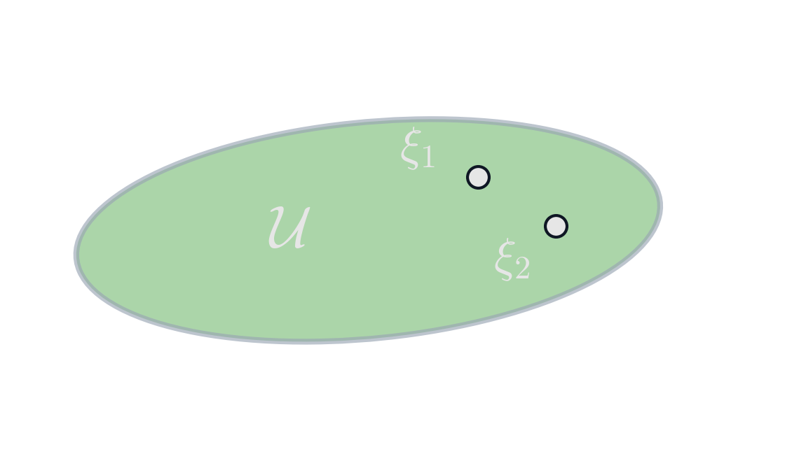
\[ \begin{aligned} \min_x\quad & f(x)\\ \text{s.t.}\quad & x\in\mathcal X(\hat\xi) \end{aligned} \]

Robust model: survive all worlds
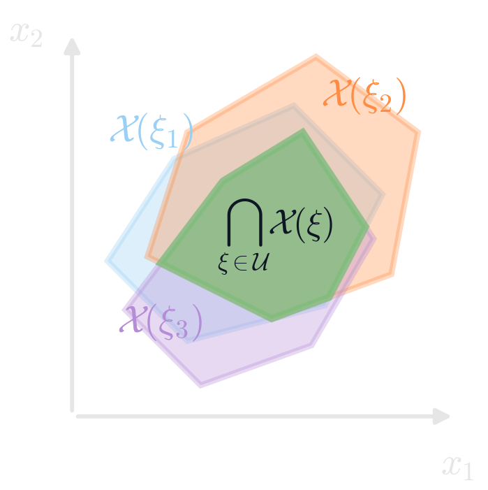
\[ \begin{aligned} \min_x\quad & f(x)\\ \text{s.t.}\quad & x\in\mathcal X(\xi) \quad \forall \xi\in\mathcal U \end{aligned} \]

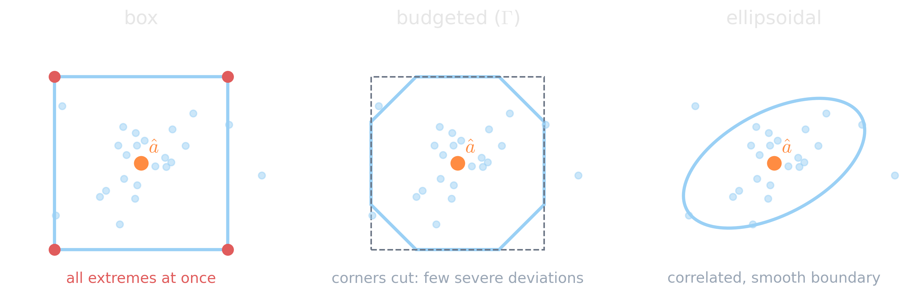
The box set: every coefficient at its worst

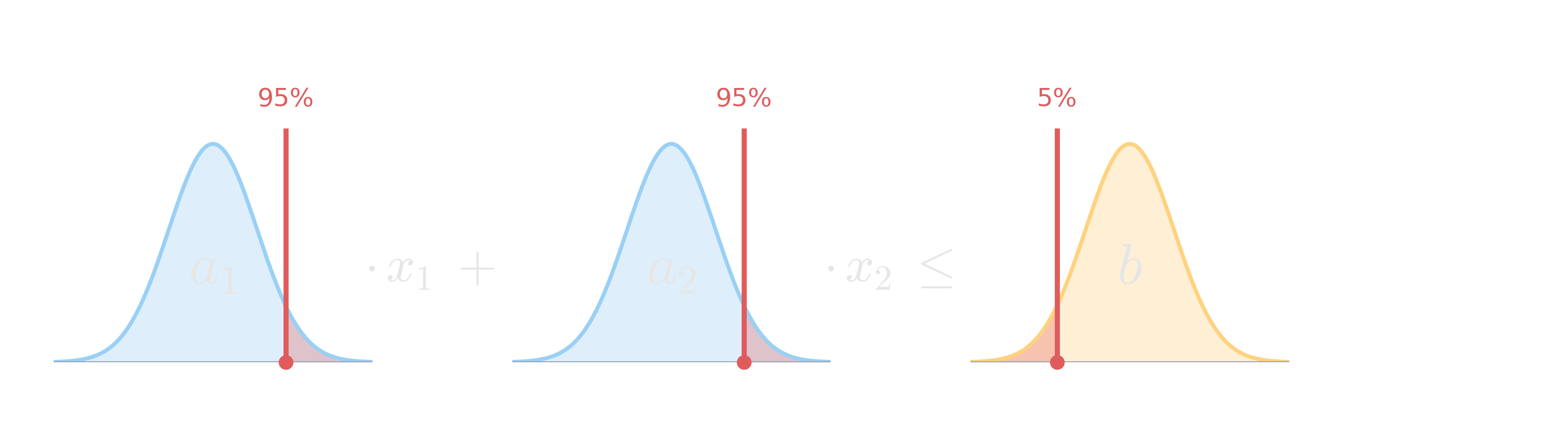
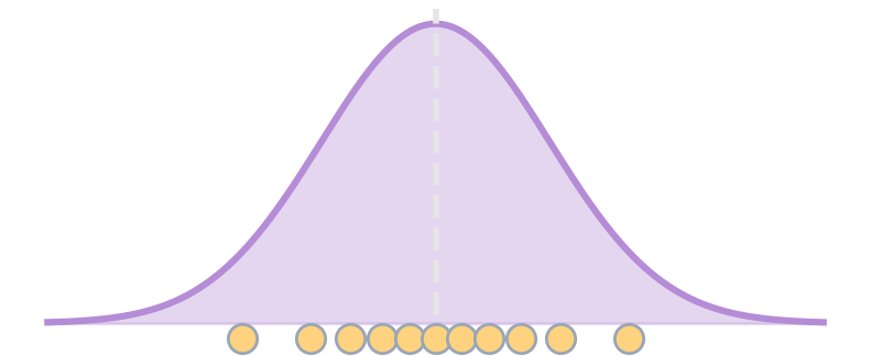
Behind every coefficient of \(a^\top x \le b\) sits a distribution, not a single number.
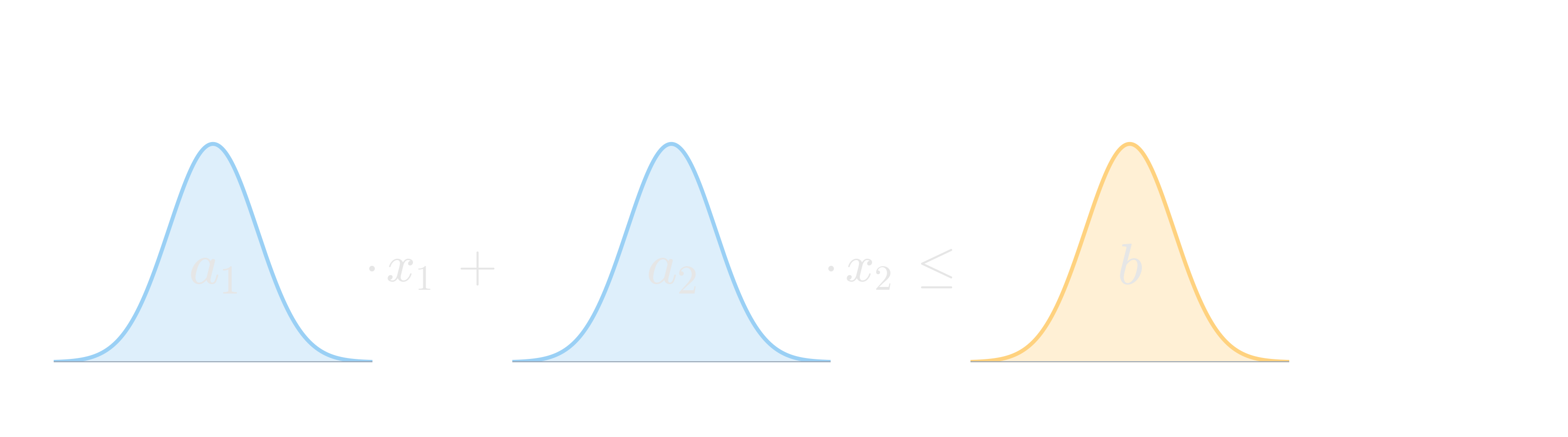
The box protects against the worst tail of every coefficient simultaneously.

Every coefficient hitting its worst value at the same time is highly unlikely. The box guards a joint scenario that almost never occurs, so it is overly pessimistic.

Central limit theorem

Recall: if \(X_1,\dots,X_n\) are independent with mean \(\mu\) and standard deviation \(\sigma\), then

\[ \frac{X_1+X_2+\dots+X_n-n\mu}{\sigma\sqrt{n}}\;\xrightarrow{\ d\ }\;\mathcal N(0,1). \]

  • Sums of many independent terms stay close to their mean.
  • The spread grows like \(\sqrt{n}\), not like \(n\).

Can we exploit this to build a tighter uncertainty set?

Protecting against fate flipping a coin

Fair coin: the fraction of heads over \(n\) flips has mean \(0.5\) and spread \(0.5/\sqrt{n}\).
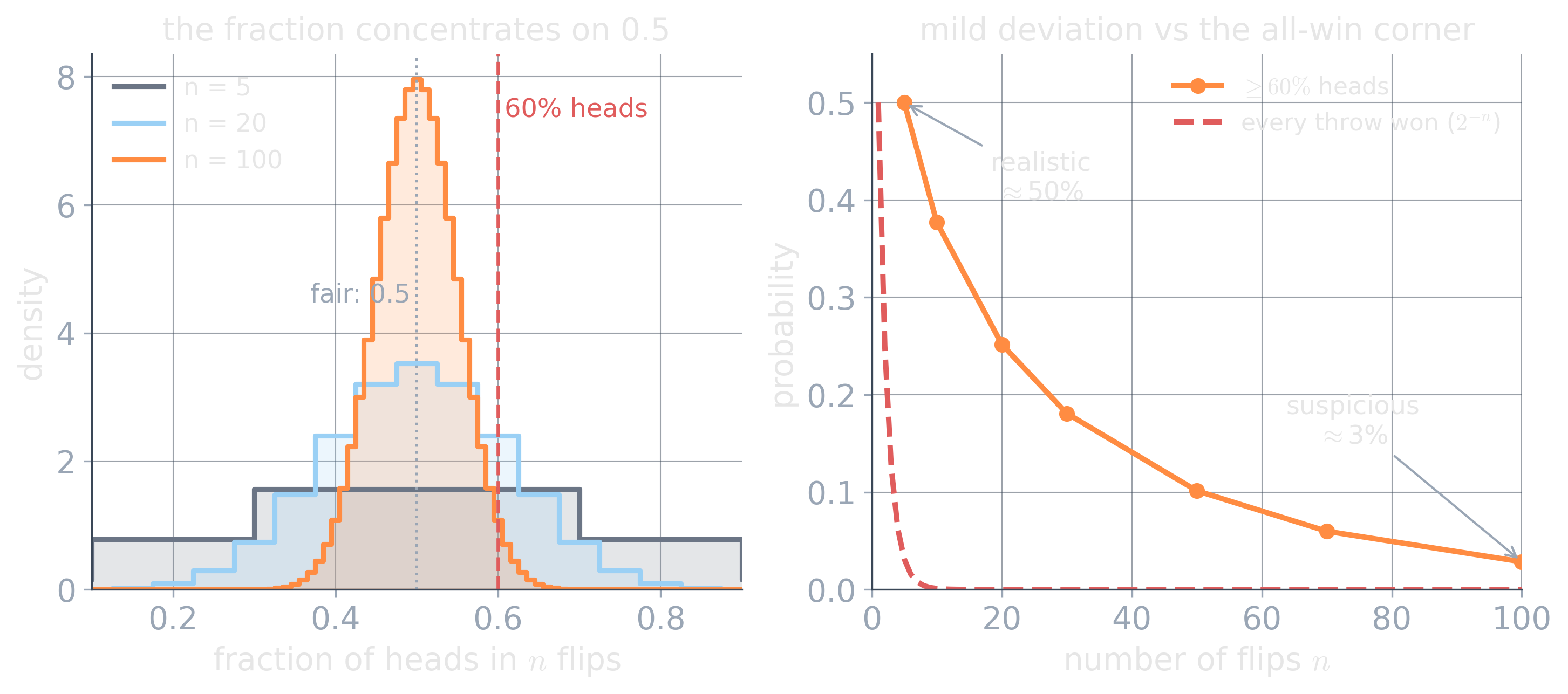
60% heads: near even odds over 5 tosses, a \(2\sigma\) rarity (\(\approx 3\%\)) over 100.

Winning every toss is the box corner: probability \(2^{-n}\). The plausible band spans a few \(\sigma\), and that width is the budget \(\Gamma\).

CLT-based uncertainty set

Bound the summed, standardized deviation from the nominal coefficients \(\hat a_i\):

\[ \mathcal U_\Gamma=\Big\{\,a:\;-\Gamma\sqrt{n}\;\le\;\sum_{i=1}^{n}\frac{a_i-\hat a_i}{\sigma_i}\;\le\;\Gamma\sqrt{n}\,\Big\}. \]

Keep a plausible interval per coefficient too (\(|a_i-\hat a_i|\le\sigma_i\)). Box plus budget give the corner-cut budgeted set.

\(\Gamma\) = standard deviations of coverage: \(\Gamma=2\Rightarrow\approx 95\%\), \(\Gamma=3\Rightarrow\approx 99.7\%\).

The coverage is asymptotic and assumes many, roughly independent terms. A few dominant coefficients or strong dependence loosen the guarantee.

The set shape is a modeling choice

Whatever the shape, it is an assumption, not a fit. Calibrate it from domain knowledge and data, then validate coverage and decisions out of sample.

The price of robustness

A larger uncertainty set gives stronger protection, a smaller feasible region, and a nominal objective that cannot improve.

protection \(\longleftrightarrow\) conservatism

Robustness is a posture, not a switch: bound the uncertain world with a set that probability can justify and an optimizer can still solve.
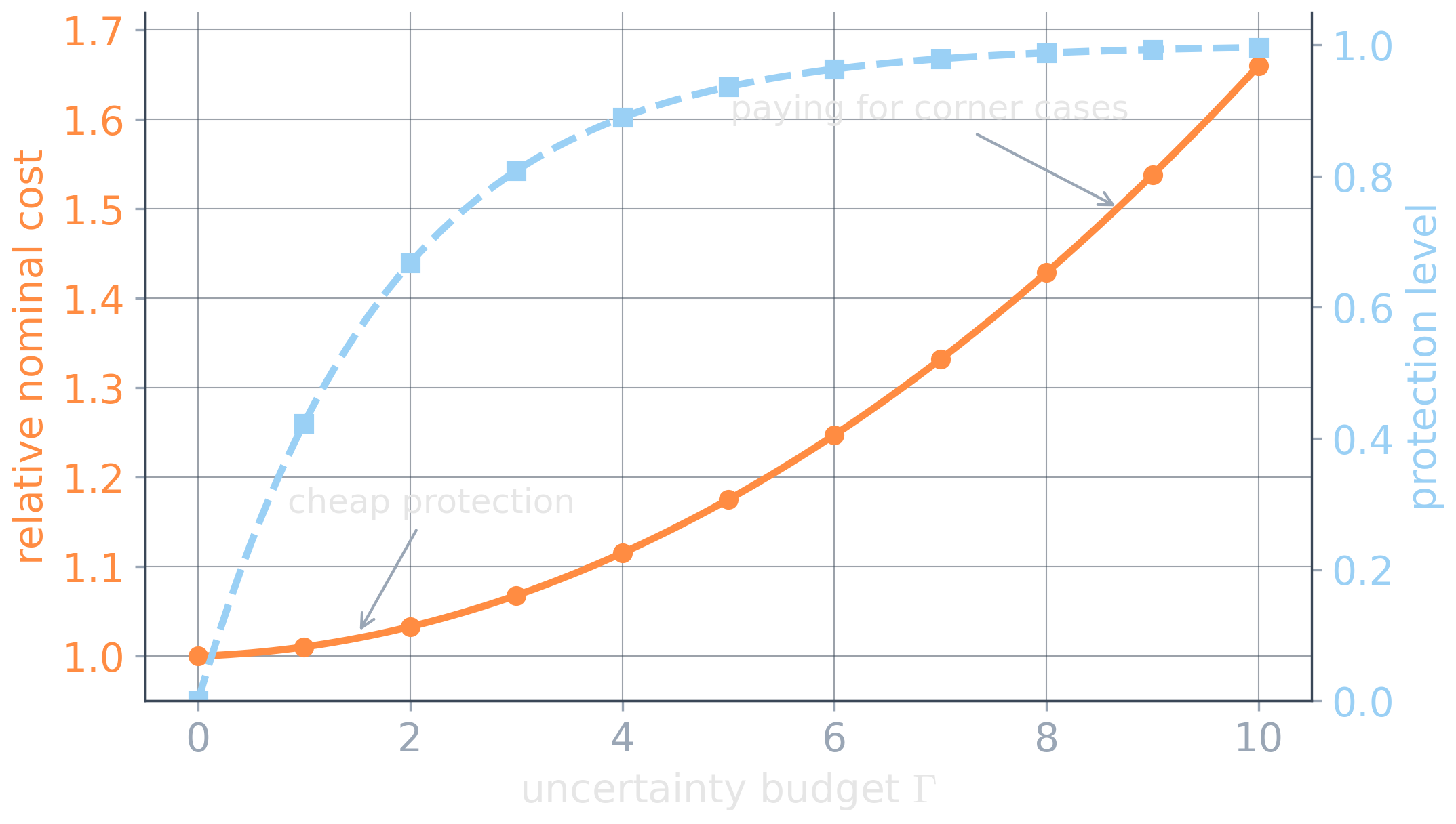
Robust Optimization & Sequential Decision-Making by Phebe Vayanos (CompSustNet)

Stochastic Optimization

Weight possible futures probabilistically. And, when possible, react after learning which future arrived.

From robust to stochastic

Robust

\[ \min_x\; \max_{\xi\in\mathcal U} c(x,\xi) \]

Protect against every realization represented by \(\mathcal U\).

Stochastic

\[ \min_x\; \mathbb E_{\xi\sim P} \big[c(x,\xi)\big] \]

Weight futures according to a probability model.

You have already solved one:

\[ \min_q \mathbb E\!\left[ C_u(D-q)^+ + C_o(q-D)^+ \right]. \]

The newsvendor optimizes one order quantity across a distribution of demands.

Weighted scenarios: several futures, one decision

In a stochastic scenario model, each scenario is a coherent possible future with a probability or empirical weight.

scenario demand weight
low 80 0.2
normal 100 0.5
high 140 0.3

For one fixed decision \(x\):

\[ \min_x \sum_{s\in S} p_s\,c(x,\xi_s). \]

The same \(x\) is evaluated across all scenarios. There is no adaptation yet.

A scenario should often represent a joint future, not independent guesses for each coefficient: demand, prices, failures, and durations may move together.

The deeper idea: recourse

Many real decisions are not made all at once.

Production planning

  1. Today: reserve capacity and staffing
  2. Tomorrow: demand is observed
  3. Then: use overtime, outsource, or reschedule

\[ x \;\longrightarrow\; \xi \;\longrightarrow\; y(\xi) \]

commit \(\;\to\;\) observe \(\;\to\;\) react

Good uncertainty handling is often about deciding what must happen now and what can wait.

Two-stage stochastic optimization

A canonical form is

\[ \min_x \left[ c^\top x + \mathbb E_\xi\big[Q(x,\xi)\big] \right], \qquad Q(x,\xi) = \text{optimal cost of reacting after observing }\xi. \]

First stage: \(x\)

  • here-and-now
  • chosen before uncertainty resolves
  • shared across futures

Second stage: \(y(\xi)\)

  • recourse
  • chosen after observing information
  • may adapt to the realized future

\(Q(x,\xi)\) is itself an optimization problem: given the commitment \(x\) and realization \(\xi\), choose the best feasible reaction.

Shared commitments, scenario-specific reactions

For finite scenarios:

\[ x \longrightarrow \begin{cases} \xi_1 \longrightarrow y_1\\ \xi_2 \longrightarrow y_2\\ \xi_3 \longrightarrow y_3 \end{cases} \]

The deterministic equivalent has the conceptual form

\[ \min_{x,y_1,\dots,y_S} c^\top x + \sum_{s\in S} p_s\,q_s^\top y_s \]

subject to common first-stage constraints and scenario-specific recourse constraints.

\[ \boxed{x\text{ is shared across scenarios}} \qquad \boxed{y_s\text{ may differ after scenario }s\text{ is observed}} \]

Nonanticipativity: no clairvoyance

Suppose capacity must be reserved before demand is known.

Wrong: scenario-specific first-stage copies \(x_{\text{low}},\; x_{\text{normal}},\; x_{\text{high}}\).

This secretly chooses today’s commitment after learning tomorrow’s scenario.

For a two-stage model, the first-stage copies must agree:

\[ x_{\text{low}} = x_{\text{normal}} = x_{\text{high}}. \]

General rule:

\[ \boxed{ \text{same information history} \;\Longrightarrow\; \text{same decision} } \]

A decision may depend only on information available when it is made.

Sample Average Approximation

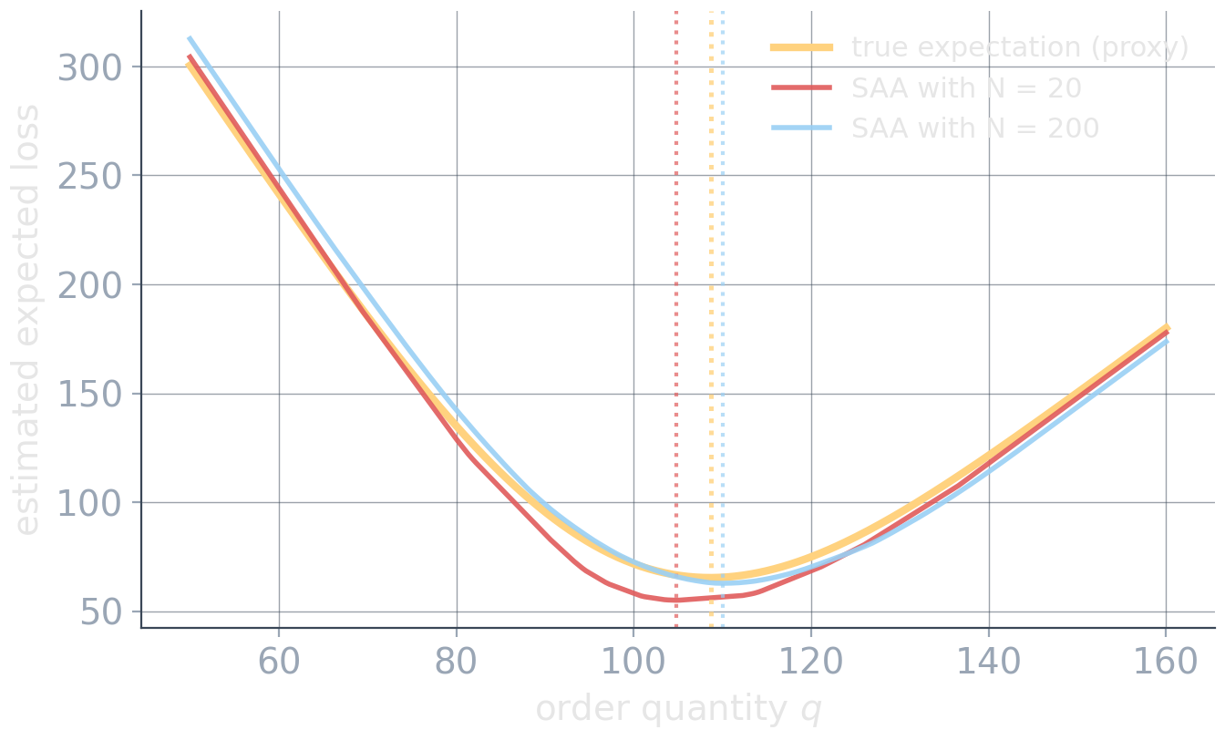
Often the expectation cannot be evaluated analytically. Suppose we have representative samples \(\xi^{(1)},\dots,\xi^{(N)}\) of the uncertainty. Replace the expectation by the empirical average:

\[ \min_x\; \mathbb E[f(x,\xi)] \quad\rightsquigarrow\quad \min_x\; \frac1N \sum_{i=1}^N f(x,\xi^{(i)}). \]

For two-stage recourse:

\[ \min_x\; c^\top x + \frac1N \sum_{i=1}^N Q(x,\xi^{(i)}). \]

Samples make the expectation computationally tangible, at the cost of sampling error and often a much larger model.

More samples reduce sampling noise

Larger samples often stabilize the empirical objective, but they do not generally make an optimization problem smooth. They also enlarge scenario-based models.

Optimize on one sample, evaluate on another

Do not trust the scenarios used to choose the solution.

\[ \text{training scenarios} \;\longrightarrow\; \text{optimize} \;\longrightarrow\; x^* \;\longrightarrow\; \text{fresh evaluation scenarios} \]

Evaluate: mean realized cost · variability · violation / infeasibility rate · tail loss · stability of the chosen decision

\[ \boxed{ \text{good in-sample objective} \;\not\Rightarrow\; \text{good stochastic decision} } \]

Expectation is not safety

Optimizing \(\;\min_x \mathbb E[c(x,\xi)]\;\) may rationally accept a rare disaster if its probability is small enough.

Risk treatment addresses the distribution of bad outcomes:

  • chance constraints: control violation probability
  • CVaR / risk measures: penalize bad-tail outcomes

Multistage stochastic programming addresses something different: repeated information arrival and repeated adaptation,

\[ x_1 \to \xi_1 \to x_2 \to \xi_2 \to x_3 \to\cdots \]

A stochastic model is not automatically safe. It is only as credible as its probabilities, scenarios, risk criterion, and information structure.

Recap

We started with one objective and trusted data. We now have a response to each.

Answering the two questions

\[ \min \{ f(x) \mid x\in\mathcal X \} \]


Quality is multidimensional.

  • Encode preferences you can defend: exchange rates, priorities, or limits.
  • Otherwise expose the trade-off and let the Pareto front decide.

Reality is uncertain.

  • Diagnose the mismatch first.
  • Choose a representation (nominal, robust, stochastic) and, separately, when decisions may adapt.
  • Validate out of sample.

Ehrgott, Multicriteria Optimization (Ehrgott 2005) · robust optimization: (Ben-Tal et al. 2009; Bertsimas and Hertog 2022) · Birge & Louveaux, Introduction to Stochastic Programming (Birge and Louveaux 2011) · decision-focused learning: (Elmachtoub and Grigas 2022)

See you next lecture

References

Ben-Tal, Aharon, Laurent El Ghaoui, and Arkadi Nemirovski. 2009. Robust Optimization. Princeton University Press.
Bertsimas, Dimitris, and Dick den Hertog. 2022. Robust and Adaptive Optimization. Dynamic Ideas.
Birge, John R., and François Louveaux. 2011. Introduction to Stochastic Programming. 2nd ed. Springer.
Deb, Kalyanmoy, Amrit Pratap, Sameer Agarwal, and T. Meyarivan. 2002. “A Fast and Elitist Multiobjective Genetic Algorithm: NSGA-II.” IEEE Transactions on Evolutionary Computation 6 (2): 182–97.
Ehrgott, Matthias. 2005. Multicriteria Optimization. 2nd ed. Springer.
Elmachtoub, Adam N., and Paul Grigas. 2022. “Smart ‘Predict, Then Optimize’.” Management Science 68 (1): 9–26.