From Model to Decision: The Analytics Lifecycle and Decisions Over Time
Algorithm Engineering — L14
Welcome
Two steps back
The model is the part you now know how to build. It is rarely the part that decides success.
Where we have been, and the two gaps left
Everything so far assumed a decision made once, from a model handed to us already framed.
Gap 1: the model is not the project.
Data, stakeholders, deployment, and adoption surround it. Ask a practitioner where projects die, and it is almost never the math.
Gap 2: decisions live in a running system.
Your output is not a one-shot answer but a policy that keeps acting: re-plan every night, re-price every week, refill when stock runs low. Information arrives between decisions.
Two lenses for the two gaps: the INFORMS Analytics Framework for the project, Sequential Decision Analytics for the stream of decisions.
Part I: The Analytics Lifecycle
Zoom out until the solver is one box among seven.
Three kinds of analytics
Sorted by the question each answers, not by difficulty.
A stack, not a menu: a prescriptive decision rests on a prediction, which rests on a description of what is going on. Optimization is the top layer.
How a Project Actually Runs
Building the model is stage 5: often just 10-15% of project time, and rarely the stage that decides the outcome.
Irv Lustig, Optimization Solution Development & Deployment
youtu.be/RA-q4lYZNvI
Seven domains of the INFORMS Analytics Framework (INFORMS 2024; Lustig and Bos-Beijer 2025). informs.org/Professional-Development/Professional-Development-Classes/INFORMS-Analytics-Framework
Domain I · Business Problem Framing
Find a question whose answer is worth money, and agree on it.
- State the problem: name the pain and a target in plain words, as a business question with its background and scope, before anyone reaches for a model.
- “Vans return after 19:00 and we pay 20% overtime. Can we get the fleet back by 18:00?”
- Identify stakeholders: sponsors, process owners, IT, influencers, end users, and each one’s RACI role (responsible, accountable, consulted, informed).
- Sponsor: operations director. Users: dispatchers (route by hand). Affected: drivers. Data owner: IT / telematics.
- Amenable to analytics?: confirm it is repeatable and data-rich enough to need a model, and name a concrete reason it might not be.
- Routing, yes. But first rule out the dull cause: too few vans is a hiring decision, not a model.
Domain I · Business Problem Framing, continued
Sharpen the question, price it, and get a signature.
- Refine until clear: turn the mood into a testable objective plus constraints, measurable and time-bound, and fix the one phrase still left vague.
- From “make delivery better” to “minimize total route time so every van is back by 18:00, no missed windows.”
- Initial business case: weigh benefit (business, societal, analytical), cost, and the baseline to beat, and name the unintended consequences, direct and indirect.
- ~15% less overtime ≈ €120k/yr (assumed); cost = build + solver + retraining; baseline = manual, 45 min/morning; side effect: daily route churn annoys drivers.
- Sponsor agreement: get a signature on the problem, the target, the budget, and what is explicitly in and out of scope.
- Ops director signs the one-sentence problem and 18:00 target; same-day re-routing is out of scope; dispatchers pilot before it is mandatory.
Domain II · Analytics Problem Framing
Translate the business question into a measurable analytics problem.
- Reformulate as an analytics problem: objective plus constraints, and its analytics type (descriptive, predictive, prescriptive).
- “Assign each stop to a van, order stops to minimize drive time, within capacity and time windows.”
- Drivers, inputs, outputs: classify each quantity: input, output, both, or neither.
- Inputs: locations, service times, capacity, traffic. Output: an ordered stop list per van.
- State assumptions: explicit and implicit, and how you’d check each held.
- Service time fixed; traffic average for the hour; every parcel fits; no breakdowns.
- Primary measures of success: split the business KPI from the model objective, which is often only a proxy and can diverge from it.
- Business KPI: overtime past 18:00, on-time %. Model objective: total drive time.
Domain II · Analytics Problem Framing, continued
Set the bar, and get buy-in before building.
- Baseline of the current state: measure today so improvement is provable.
- Replay last month’s manual routes: 6.2 overtime h/van/week, 91% on-time. That is the number to beat.
- Risks and mitigations: anticipate what could sink it and how you’d blunt each: data limits, model bias, ethical risk, over-reliance on generative AI.
- Dispatchers reject “weird” routes → human-in-the-loop + explanations. Bad addresses → validate geocoding; a model fit to old routes can bake in old bias.
- Sponsor agreement on the framing: confirm this framing still delivers the promised value, and align every RACI party on it before any build.
- Ops director agrees success is overtime cut against the replayed baseline, not “faster” in the abstract.
Domain III · Data
Get the right data, and make it trustworthy.
- Identify and prioritize data needs: rank them, and flag sensitive fields.
- Must-have: addresses, time windows, capacity. Nice-to-have: live traffic.
- Identify and analyze sources: where each field lives, in what form and what condition, and who owns it (owner, steward, custodian).
- Orders in the order system; traces from telematics; capacities in a spreadsheet.
- Data management plan: refresh, storage, access, and security, sized to the four Vs (volume, velocity, variety, veracity).
- Nightly export of tomorrow’s stops; addresses geocoded once and cached.
- Acquire data: a real extract, with lineage and version control.
- Pull last month’s orders and traces; build on real routes, not toy data.
Domain III · Data, continued
Clean it, understand it, document it, and loop back.
- Clean, harmonize, validate: the standard defects: missing, duplicate, mistyped, corrupt, default, out-of-range.
- Geocode addresses, drop duplicates, join each stop to its van, flag the 3% with no location.
- Assess quality and relationships: score quality (accuracy, completeness, consistency, timeliness, validity, uniqueness, outliers), then profile structure.
- Service time varies 2× by parcel type; “traffic” is really the hour of day.
- Document and report findings: record tables, fields, quality, assumptions.
- A data doc: every table and field type, the 3% geocoding gap, and how it was handled.
- Validate and update the problem statements: loop back if the data changes what’s feasible.
- No reliable time windows → soften “no missed windows” to “minimize total lateness.”
Domain IV · Methodology (Approach) Framing
Choose the method and the stack that fit the problem and the data.
- Determine candidate methods: across the analytics types (descriptive, predictive, prescriptive); routing is prescriptive.
- A capacitated vehicle routing problem with time windows: an exact IP, or metaheuristics.
- Evaluate and select, given data and resources: fit to the data, the time, and the team’s skills; weigh technical vs business cost, benefit, risk.
- 300 stops nightly in minutes → a metaheuristic; keep the exact model for tiny depots.
- Understand the solution architecture: sketch how data flows in and out.
- Nightly batch: export tomorrow’s stops → solve → push routes to the driver app by 05:00.
- Evaluate and select the technology stack: pick tools and solver: cloud or on-prem, open-source or proprietary; a spreadsheet can be right, not here.
- Python with a routing solver; the order database for stops; a small service feeding the app.
Domain V · Analytics / Model Development
Build the model, and prove it works.
- Design the model structure: variables, objective, constraints on paper first; a prescriptive model needs decision variables, constraints, an objective, a predictive one dependent and independent variables.
- Vars: which van visits each stop, in what order. Objective: total drive time (proxy) plus a lateness penalty. Constraint: van capacity. Overtime past 18:00: a KPI, not a hard cap.
- Build one or more models: implement it, maybe as competing variants, and check nothing is missing or double-counted in the formulation.
- A base router; a variant that may defer a stop to tomorrow when the fleet is overloaded.
- Run, verify, evaluate: check it solves in time, the routes make sense, and no biased or unethical outcome slipped in.
- Solves in 90 s for 300 stops; total drive time down 12% versus the baseline on last month’s data.
Domain V · Model Development, continued
Tune it to reality, connect it, and write it down.
- Calibrate with client input: tune parameters so output matches reality; trace each client complaint to a data or model cause.
- Dispatchers: “15 min at this hospital, not 5.” Fix per-stop service times, then re-solve.
- Integrate multiple models if needed: connect models when one feeds another, and resolve their conflicts and synergies.
- A demand forecast picks tomorrow’s likely stops; the router plans them. Two models, one pipeline.
- Document model findings: write the math, assumptions, limitations, and constraints, in plain terms for a non-technical audience.
- A model doc: objective, every constraint, the constant-service-time assumption, and what it cannot do.
Domain VI · Deployment
Ship it into the business, not just onto a server.
- Business validation: confirm with the business that it solves the real problem, not a proxy, and surface any ethical risk before it ships.
- Run a week of real days in parallel; dispatchers compare the model’s routes to their own.
- Validation report: write up what validation showed, the gaps included, with a plain-language summary for the sponsor.
- Report: overtime down 14% on the pilot week; two depots still need manual overrides.
- Sponsor agreement to proceed: get the green light to deploy.
- Ops director signs off on rollout to the pilot depot after seeing the validation numbers.
Domain VI · Deployment, continued
Specify it, stand it up, and verify it on live data.
- Requirements for the deployed solution: model, usability, system, and business needs, documented so it can be reused if the business changes.
- Routes ready by 05:00; a dispatcher can lock or edit a stop; a fallback if the solve fails.
- Support implementation and testing: help stand up, load-test, and harden production, and name who owns it once live.
- Integrate with the driver app; load-test the nightly run; test the “solver failed” fallback path.
- Validate production data flows: verify it works on live data end to end, and pin down which sources must stay synchronized.
- Watch the first live weeks; confirm the nightly export still matches the format the model assumes.
Domain VII · Analytics Solution Lifecycle Management
Keep the benefit alive after everyone moves on.
- Track performance: monitor the KPI over time; define what “acceptable” is and what could drift it out of range.
- A dashboard of weekly overtime and on-time %, with an alert if overtime creeps back up.
- Recalibrate and maintain: retune as the world drifts, weighing the opportunity and the risk of each change before you ship it.
- A new depot and two more vans next quarter: re-tune capacities and service times.
- Support training: train three audiences, analytics, IT, and business users, so each can run it.
- Onboard new dispatchers; document how to override, and when to trust the routes.
Domain VII · Lifecycle Management, continued
Re-earn the business case, and stay hand-off-ready.
- Validate the business case over time: confirm it still delivers, and isolate the benefit actually attributable to the solution.
- Six months on, is overtime still down €120k/yr, or has the benefit quietly eroded?
- Analyze side effects: watch for unintended consequences that surface only over time, including an ethical issue not visible in the data.
- Drivers dislike routes that change daily → keep routes stable where the cost difference is small.
- Keep documentation maintained: stay hand-off-ready as staff turn over, and record which lifecycle activities to monitor.
- No obfuscated code, model math kept current, so the next team can take it over.
The same seven stages, in the wild
Every large deployment is a full walk of the seven stages, not a clever model in isolation.
- UPS ORION (delivery routing): ~3 years of field testing, hundreds of deployment staff, tens of thousands of drivers before it paid off. (Holland et al. 2017)
- HP print forecasting (18,000+ products, 170+ countries): a machine-learning model living inside a human-in-the-loop workflow, not replacing it. (Harshvardhan et al. 2025)
- U.S. Census MOJO (2020 nonresponse follow-up): ML plus optimization replaced a paper process; now extending to 90+ surveys. (Adams et al. 2023)
In each, the win came from framing, data, deployment, and lifecycle; the model was a minority of the effort. The framework is really a handoff-control system: it stops work dying in the seams between sponsor, experts, analysts, data, IT, and operators.
It is a cogwheel, not a pipeline
Stages feed backward as often as forward. A discovery late invalidates an assumption early.
Real engagements rarely start at stage 1:
- “We have data, what can we do?” → starts at 3. Walk backward or die by dashboard.
- “We already bought the optimizer.” → starts at 4. The hardest entry to recover from.
- “Keep the existing solution running.” → starts at 7.
Enter mid-framework? Walk backward first: sponsor-aligned problem, KPI, baseline, owned data. Then go forward.
Where projects actually die
The math is right, but nobody uses it.
Stage 6 is half technical, half organizational, and the organizational half is where good models go to die:
- A plan the optimizer proves optimal, that the planners do not trust, is not deployed.
- No fallback for an infeasible or late solve means the first bad night ends the project.
- No internal champion with authority means the change stalls the moment it inconveniences someone.
Deployment is not shipping a binary. It is shipping a change in how people work. Budget for the second half or the first half is wasted.
Twenty risks, and most are not the math
The Princeton 20 pre-mortem (Princeton Consultants): score each factor green, yellow, or red.
Environmental: the organization
- Sponsoring business: healthy, or shaky?
- Sponsoring executive: owns the process?
- Business process: mature, or brand-new?
- Decision-support culture: uses models?
- Decision scope ★: one sentence, or fuzzy?
- KPIs: measurable, with a baseline?
- Value proposition ★: quantified per year?
- Resource availability: key people free?
- Other initiatives: contending for the SMEs?
- User engagement: users under the sponsor?
Technical: the model and stack
- Existing model: replacement, or greenfield?
- Application novelty: proven elsewhere?
- New technologies: proven, or vaporware?
- Decision scoring: can you write a formula?
- Business rules: codifiable as math?
- Decision data: sufficient and clean?
- Software tools: team-owned and mature?
- Speed: is faster actually worth money?
- UX: does it drive optional adoption?
- Process maturity ★: shipped to production?
Environmental factors (Sashihara 2019a) · technical factors (Sashihara 2019b).
If you assess only three risks
Of the twenty, three dominate the outcome.
Decision Scope
Can you state the decision in one sentence? Fuzzy scope across many functions becomes an unbounded project.
Value Proposition
What is it worth per year, against what baseline? “Efficiency” is not a value. Dollars, hours, throughput are.
Process Maturity
Has this org shipped and sustained an optimization system before? A perfect model on an immature org is wasted.
Thirty minutes with the sponsor, these three questions, in order. A red on any of them should reshape the engagement, not be papered over.
Interview with Irv Lustig (Princeton Consultants), who helped shape the framework — real client stories: Identifying and Mitigating AI Project Risk. youtu.be/j1WTCLQfTCY
The three dominant risks of the twenty (Lustig 2025).
Part II: Sequential Decisions Analytics
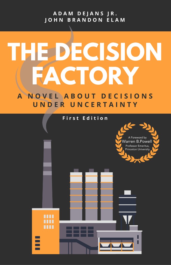
This entire example follows the arc of The Decision Factory (DeJans & Elam), which we drew on heavily. Recommended reading for how optimization actually lives inside real operations, told as one continuous story.
The setting: Ward 5-West
We built and deployed a nurse-rostering optimizer for a 30-bed ward: a clever decomposition returns a provably optimal roster in under an hour. A month later the hospital calls us back: the nurses are furious and want to roster by hand again.
The problem we were handed:
- Classical rostering: staff every shift to satisfy regulations, contracts, and stated preferences.
- Short-handed, three priced levers: overtime, borrow a nurse from another ward, or call an agency. Prices are accurately known, given to us by management.
- Understaffed, the cost escalates with severity: penalty, then turn patients away, then close the ward. These we can only roughly guess, but we have numbers.
- Demand is predictable: no ER, so the ward plans well ahead.
The data is honest, and the solver is optimal. What is likely going wrong?
What we delivered, and why it fails
We shipped the tool: the optimal shift assignment for the next two weeks. On our metrics it beats the ward’s historic manual schedules.
The nurses tell us the plans just don’t work.
- We had already built in robustness: slack and buffers on the tight shifts.
- It still shatters after the first sick call, and the day ends in a scramble.
- Turn robustness up, and the model reports there is not enough staff to guarantee it.
- Management: “we have always coped at this staffing level.”
The solver is fine. The horizon is the problem: no static two-week plan survives two weeks of surprises, and the surprises arrive after we commit.
Two fixes, both rejected
Both keep the same tool and only move the horizon.
Shorten it: plan two days ahead. Short enough that the forecast holds.
Rejected: nurses cannot run their lives on two days’ notice, not with childcare, second jobs, and appointments to arrange.
Keep two weeks, but re-solve whenever something major changes. Accepted for a trial.
Rejected too: every re-solve rewrites the whole roster. A €40 saving moves a nurse off the Thursday she planned around. The schedule churns, and still no one can plan ahead.
Both are still plans: one accurate but unlivable, the other livable in name only. Moving the horizon just trades responsiveness against stability. We need to step back.
A plan is not a policy
The failure is not the optimizer. It is the job we gave it.
A plan
A fixed sequence \((x_0, x_1, \dots, x_T)\), committed at \(t=0\), before any information arrives.
Optimal only for the one future assumed at solve time.
A policy
A function from what you know now to a decision: \[x_t = X^\pi(S_t)\]
Defined for every future, because it consumes information as it arrives.
The published roster is a plan \(\bar{y}\); operating the ward needs a policy \(X^\pi\). Re-solving on every change was already a policy, and a step in the right direction: it consumed new information. It just optimized each step in isolation, blind to the cost of change. So the goal is not a better \(\bar{y}\), but a better \(\pi\), one that values stability too.
Frame the problem: three questions first
Answer these before deciding how to solve it.
- What are the decisions, and who owns them?
- How do we measure quality?
- What uncertainty affects performance?
Confucypus says: a mind narrowed to what solves easily soon loses sight of what is worth solving. Reach for the method first, and it chooses the problem for you.
Question 1: the decisions, and their owner
What are the decisions, and who owns them?
Two recurring decisions:
What we tell the nurses — the roster we publish and commit to. They arrange their lives around it and expect it mostly honored.
What we do when things change — staff the next shift when it comes up short: do nothing, pull a float nurse, offer overtime, reassign across wards, or book an agency nurse.
Owner: the charge nurse.
- accountable for patient safety
- authority to override the system
- works the levers by hand: phones nurses, coaxes overtime, chases agency
- must be in the room while it is built
A system built without its owner will be ignored, and it should be.
Question 2: how we measure quality
How do we measure quality?
Not one number. Six that pull against each other:
- labor cost: regular, overtime, agency
- coverage: shifts at or above the safe ratio
- fairness: how the ugly shifts and overtime spread across nurses
- preference satisfaction: honored requests
- stability: how much the published roster survives contact with the week
- tail safety: the worst shifts, not the average one
Resist collapsing these into one weighted sum. Hidden weights hide what you give up. We will surface the trade-offs instead.
Question 3: what is uncertain
What uncertainty affects performance?
Everything the world reveals between one shift and the next:
- sick calls and no-shows
- census: admissions and discharges
- patient acuity
- float and agency availability, when you reach for them
- whether offered overtime is accepted
“Offering is not getting.” These become the exogenous information \(W_{t+1}\) in the frame, the reason a fixed plan cannot hold.
The five elements for the ward
| Element | Symbol | For Ward 5-West |
|---|---|---|
| State | \(S_t\) | roster commitments, who is out today, census/acuity forecast \(\hat{D}_t\), fairness + hours ledgers, float/agency status |
| Decision | \(x_t \in \mathcal{X}(S_t)\) | float / overtime / reassign / agency / accept short (legal rest, skill mix, availability) |
| Exogenous info | \(W_{t+1}\) | new sick calls, admissions & discharges, acuity, realized float/agency, overtime acceptance |
| Transition | \(S_{t+1}=S^M(S_t,x_t,W_{t+1})\) | apply staffing, advance census, roll hours + fairness; overtime tonight rest-locks a nurse tomorrow |
| Objective | \(\min_\pi \mathbb{E}\sum_t C(S_t, X^\pi(S_t), W_{t+1})\) | labor + convex shortfall + fairness + stability |
The catch is twofold: \(W_{t+1}\) is revealed only after we commit, and our own decision reshapes the next feasible set \(\mathcal{X}(S_{t+1})\). A fixed plan answers to neither; a policy answers to both.
A first real policy, and the trust problem
The frame moves the target: judge the system over time, not the objective of one isolated solve.
So we build a real policy: re-solve daily on a rolling horizon, and penalize changes to the published roster. Responsive to today, stable for tomorrow.
On paper, the objectives look great again.
“Looks great on paper” is what we said last time. We have spent our trust; this time we need proof before it touches a ward. How do we verify a policy without experimenting on real nurses?
Building a simulator
We cannot tune on the live ward: every experiment is paid in real missed care. So we build a simulator, a wind tunnel and not a forecast: it does not say who is sick next Tuesday, it shows how a policy behaves across many plausible futures.
Feed it from historic data: resample past sick calls, admissions, and acceptances into many synthetic months, and score the policy’s average cost.
The data is biased (generated under the old manual policy, not ours) and correlated (flu waves cluster, a full ward stays full). Treat draws as independent and you hide the tail risk that actually hurts.
Resample in blocks to preserve day-of-week and seasonal structure, and validate against held-out history. The lab is a guide, not truth.
The laboratory in action
One simulated week under the tuned daily-resolve policy. Read the second row:
| Shift | Gap | Decision | Revealed | Result | Cost |
|---|---|---|---|---|---|
| Mon-D | 1 | pull 1 float | +2 admits | covered | €320 |
| Mon-N | 1 | accept 1 short | quiet | 1 short | €500 |
| Tue-D | 2 | float + OT | quiet | covered | €800 |
| Tue-E | 1 | reassign from Day | 2 discharges | covered | ~€0 |
| Wed-D | 2 | float + agency | quiet | covered | €1040 |
Agency would cover Mon-N — for €720; the tuned policy takes the €500 shortfall instead. The lab shows you that behavior, and its price, before the policy ever runs a real ward — so you can accept it, or re-tune.
Monte Carlo: from one path to an estimate
One sample path is an anecdote. We judge a policy by its average over many.
Monte Carlo: estimate an expectation you cannot compute in closed form by sampling and averaging. Draw \(N\) independent paths \(\omega_1, \dots, \omega_N\), run the same policy on each (the same!), and average its cost:
\[\bar F^\pi \;=\; \frac{1}{N}\sum_{i=1}^{N} \sum_t C\big(S^i_t,\, X^\pi(S^i_t),\, W^i_{t+1}\big) \;\xrightarrow{\;N\to\infty\;}\; \mathbb{E}\Big[\textstyle\sum_t C\Big]\]
Noise. The score is itself a random estimate; its standard error shrinks like \(1/\sqrt{N}\). To halve it, quadruple the paths.
\(C\) evaluates the decision against the realized outcome \(W_{t+1}\), unknown at decision time and, thus, can only be evaluated in hindsight/simulation and cannot be directly optimized for.
The forecast is a distribution
The census forecast is not one number. It is a distribution: a spread of possible nights, with a heavy tail where several things go wrong at once.
Staff to the mean and you look efficient, until a fat-tail admissions night lands you deep in the convex part of the shortfall cost. The optimizer does not average your forecast error, it amplifies it: it pushes hard against whichever constraint the wrong number moved.
So we score on the tail, not the mean: \[\mathrm{CVaR}_{95} \;=\; \text{average cost over the worst } 5\% \text{ of nights}\]
When being short hurts far more than being spare, the mean is the wrong target. And better forecasting will not save you: the amplification lives in the decision, so the policy must carry the whole distribution through and price the tail, trading a little more on an average day for far less damage on the bad ones.
Don’t hide the trade-offs
Cost, safety, fairness, and preferences conflict. A single weighted sum buries what you give up. Surface the frontier instead.
The optimizer shows what is possible. Fairness to the worst-treated nurse and tail risk are their own axes. The owner chooses the point.
The honest baseline: an escalation ladder
On paper our plan won; in the ward, the nurses’ by-hand routine held up better. So make it the baseline: interview the charge nurse, cross-check the data, write her rule down.
When a shift is short, escalate until the gap closes:
- fill from the float pool, up to buffer \(\theta_{\text{float}}\)
- else offer overtime, up to \(\theta_{\text{OT}}\) hours
- else book agency, if lead time \(\ge 4\)h
- else accept the shortfall, and let the simulator price it
We trust the structure, not their exact numbers. Each threshold \(\theta\) becomes a hyperparameter the simulator tunes. Often the rule was right, but the cutoff should have sat one step higher.
Tuned honestly, this is a real baseline: a direct map \(x_t = \pi(S_t; \theta)\). Anything fancier must beat it, not a strawman.
Powell’s families of policies
More complex does not mean better: a fancier class can be too slow to compute in the pre-shift huddle and too opaque for the charge nurse to trust.
The CFA may look close to the original model, but it should usually carry hyperparameters that bias its coefficients to better approximate the true cost \(C\), instead of staying true to the costs we were handed.
Meta-optimization: an optimizer over optimizers
\(\displaystyle X^\pi(S_t \mid \theta) \;=\; \arg\min_{x}\ \tilde{C}(S_t,\, x;\, \theta)\)
Deployment is the start, not the end
We did not build a roster. We built a decision system: simulator, policy, tuning, metrics.
- The offline-tuned float buffer runs a little small in the real ward (sim-to-real gap); production runs more conservative.
- Re-tune each season; let θ differ by context (ICU vs. general, weekday vs. weekend).
- Log every decision: “why agency tonight?” must have an answer.
- Use an LLM to build the policy (draft constraints from the contract, explain a recommendation), not to be the policy. When it is time to decide, use the solver.
Cheapest move of all: walk the ward. A good self-swap rule may dissolve half the gaps before any solver runs.
Go deeper: the source of this vocabulary
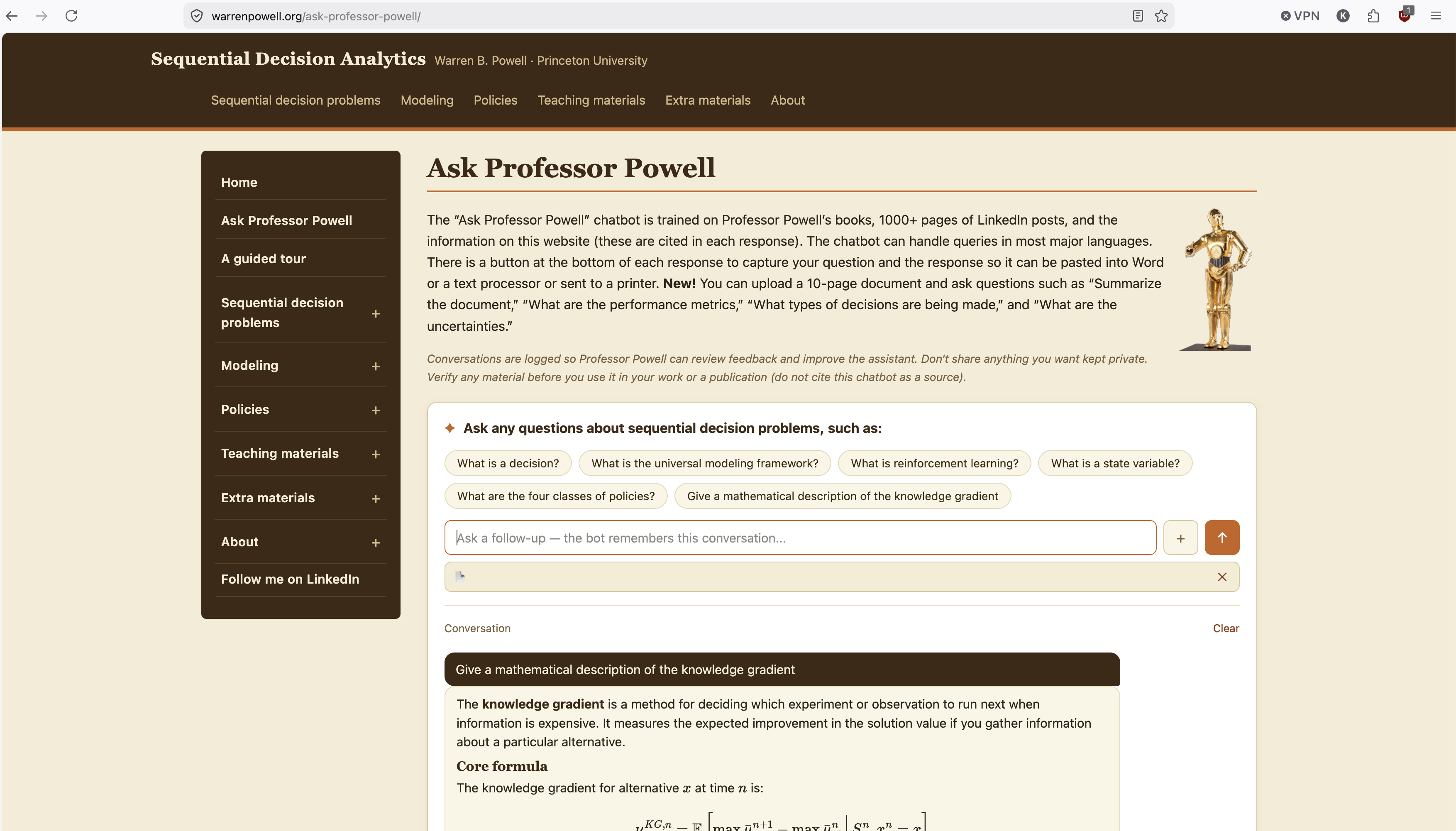
The five elements and the four policy classes are Warren Powell’s framing.
warrenpowell.org collects it all: the framework, a shorter free book, and code.
It even hosts a chatbot trained on his books and posts. Its own suggested questions are this chapter’s vocabulary: “What is a state variable?”, “What are the four classes of policies?”
Powell, Reinforcement Learning and Stochastic Optimization (Powell 2022) · warrenpowell.org/ask-professor-powell
Recap
Two steps back, two frameworks to take forward.
The two lenses, together
The project lens
Your solver is stage 5 of 7. Projects die at deployment, not in the math. Assess scope, value, and maturity before you model.
The time lens
Decisions repeat under new information. Write the five elements, choose a policy among four classes, then tune it in the simulator: an optimizer over optimizers, aimed at the real cost.
Both lenses agree: the hard part was never the solve. It is the framing around it, and the sustaining after it.
See you next time
References
Algorithm Engineering SS 2026 — L14 Analytics Lifecycle & Sequential Decisions