Performance Engineering in Practice

Algorithm Engineering — T01

Dr. Dominik Krupke

Performance Engineering in Practice

We know why code gets slow. This tutorial is about how to react.

Block 1: Find the bottleneck. Block 2: Fix the bottleneck.

Block 1: Find the Bottleneck

Before tuning anything, we need two guardrails: Amdahl’s law and “premature optimization is the root of all evil.”

Amdahl’s law: know the ceiling

If fraction \(p\) of runtime can be improved by factor \(s\), then

\[ \text{speedup} = \frac{1}{(1-p) + \frac{p}{s}} \]

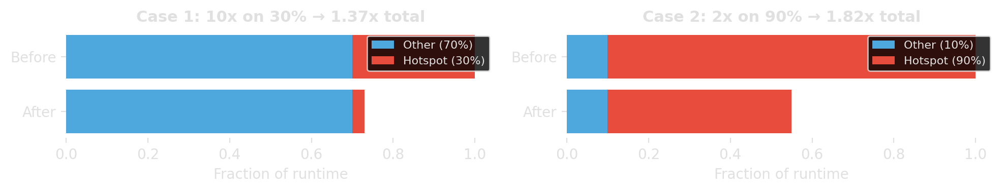
Speed up the part that dominates runtime, not the part that looks embarrassing.

“Premature optimization is the root of all evil”

“We should forget about small efficiencies, say about 97% of the time: premature optimization is the root of all evil. Yet we should not pass up our opportunities in that critical 3%.”

Donald Knuth, “Structured Programming with go to Statements”, ACM Computing Surveys, 1974. (Knuth 1974)

This quote does not mean “performance does not matter.” It means: optimize after you know where the real bottleneck is.

Photo: Alex Handy, CC BY-SA 2.0

Observability: Basic Logging

Before profilers, try the simplest thing that could work.

Start with phase markers

import logging

logging.basicConfig(
    level=logging.INFO,
    format="%(asctime)s %(message)s",
    datefmt="%H:%M:%S",
)
log = logging.getLogger("solver")

log.info("Loading instance: nodes=%d, edges=%d", n_nodes, n_edges)
# ... loading code ...
log.info("Computing greedy upper bound")
# ... heuristic code ...
log.info("Starting solver")
# ... solver code ...
log.info("Done")

The logger already adds timestamps. That is often enough to identify the slow phase.

What the timestamps reveal

16:58:12 Loading instance: nodes=500, edges=12340
16:58:12 Building graph
16:58:12 Graph built: nodes=500, edges=12340, density=0.10
16:58:12 Computing greedy upper bound
16:58:16 Upper bound found: colors=12
16:58:16 Starting solver
16:58:18 Solver finished: colors=8, optimal=True
16:58:18 Writing solution
16:58:18 Done

The “quick” heuristic is the bottleneck — 4 seconds, while the actual solver took only 2. That is where we need to speed things up.

Add structural context

log.info("Graph built: nodes=%d, edges=%d, density=%.2f",
         n_nodes, n_edges, density)
log.info("Cliques enumerated: count=%d, max_size=%d", n_cliques, max_size)
log.info("Constraints generated: %d", n_constraints)

Without input-size context, runtime logs are much harder to interpret.

Log structural statistics at natural boundaries: input size, graph size, iteration counts, constraint counts.

Controlling verbosity per component

# Each module gets its own logger
log_model = logging.getLogger("solver.model")
log_heur  = logging.getLogger("solver.heuristic")

# Use levels to express importance
log_model.info("Variables: %d, constraints: %d", n_vars, n_cons)
log_model.debug("Constraint matrix density: %.4f", density)
log_heur.warning("Greedy coloring exceeded timeout")

# Dial verbosity up or down per component
log_model.setLevel(logging.DEBUG)     # loud — investigating model size
log_heur.setLevel(logging.INFO)       # normal

Leave log calls in the code permanently. Dial verbosity up when investigating, down for production runs.

Guard expensive log computations

# Bad: computes the histogram even when DEBUG is off
log.debug("Degree histogram: %s", compute_degree_histogram(graph))

# Good: skip the expensive call entirely
if log.isEnabledFor(logging.DEBUG):
    log.debug("Degree histogram: %s", compute_degree_histogram(graph))

log.debug(...) skips formatting, but Python still evaluates all arguments before the call.

Guard with isEnabledFor() when an argument is expensive to compute.

Good code has logging — especially in production

phase markers let you pinpoint issues without reproducing them locally
add progress logs inside long loops (every N items, not every item)
use them to see scaling behavior and estimate remaining runtime

Logging tells you which phase is slow. The structural stats often tell you why at a high level. Only then do you reach for finer-grained tools.

Profiling

Logging tells us where to look. Profilers tell us how the cost is distributed inside the code.

Two big families

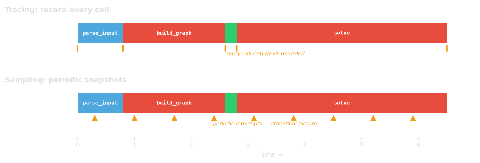
Tracing / instrumentation

record every call or event
exact call counts, higher overhead
Python example: cProfile

Sampling

interrupt periodically
statistical estimate, lower overhead
Python example: Scalene

What does “time” even mean?

CPU time: time while the program is actually running on CPU
wall-clock time: elapsed real time, including waiting
on-CPU profiles can miss I/O waits and blocking
mixed Python/native systems may need a split like Python vs native vs system

If a Python program spends a lot of time waiting or inside native libraries, the profiler must match that reality.

A practical rule of thumb

start with logging to find the slow phase
use Scalene for line-level Python vs native insight
use cProfile when you want exact call counts and call paths
if the hotspot is in native code, use native profilers (perf, VTune)

Start broad and cheap. Go narrower only where the evidence points.

cProfile: when you want exact call counts

python -m cProfile -s tottime my_script.py       # whole script
python -m cProfile -s tottime -o prof.dat my_script.py  # save for pstats
python -m cProfile -s cumtime my_script.py        # sort by cumulative

   ncalls  tottime  percall  cumtime  percall filename:lineno(function)
     1225    3.712    0.003    3.712    0.003 solver.py:42(build_graph)
        1    1.204    1.204    1.204    1.204 solver.py:89(solve)
     1225    0.847    0.001    0.847    0.001 solver.py:31(distance)

build_graph called 1225 times — if you expected once, that is the bug. Trust call counts from cProfile. Treat timing as approximate; tracing adds overhead.

cProfile: targeted profiling

# Profile just one function call
import cProfile
cProfile.run("build_graph(data)", sort="tottime")

# Profile a specific section with the context manager
with cProfile.Profile() as pr:
    result = build_graph(data)
    solution = solve(result)

pr.print_stats(sort="tottime")     # print to stdout
pr.dump_stats("profile.dat")       # save for later analysis

         2374431 function calls (828274 primitive calls) in 0.757 seconds

   Ordered by: internal time

   ncalls  tottime  percall  cumtime  percall filename:lineno(function)
   206534    0.514    0.000    0.514    0.000 cp_model.py:537(add_all_different)
1752679/206535    0.214    0.000    0.221    0.000 profile_solver.py:39(_extend)
   206535    0.012    0.000    0.232    0.000 profile_solver.py:34(enumerate_all_cliques)
        1    0.010    0.010    0.242    0.242 cp_model.py:333(new_int_var)

Scalene: when you want line-level insight (wall-clock, Python/native split)

pip install scalene
python -m scalene --html --program-path . --output profile.html my_script.py

--program-path . — only profile your code, not libraries (crucial!)
--html --output profile.html — generate a browsable HTML report
without --program-path, the output is dominated by library internals

Reading Scalene output

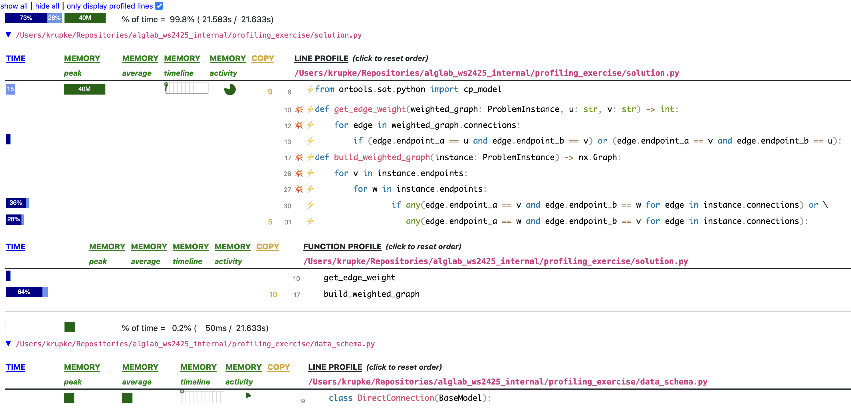
For each file, Scalene shows per-line and per-function time. Here, build_weighted_graph takes 64% — and line 30 alone takes 36%.

C++ profiling with `perf`

Profiling C++ is more painful than Python — but the payoff is a view all the way down to the hardware.

perf reads the CPU’s own counters: cycles, cache misses, branch mispredictions
You see not just where the CPU spent time, but why it spent it there
No code changes, no recompile beyond -g for symbols

Walkthrough example: examples/perf_record/

`perf` answers two questions

What kind of bottleneck is this? — compute, memory, branches, kernel, waiting
- count events across the run → perf stat
Where in the code does it land? — function, line, call path
- sample the program counter → perf record

Full program → perf record first to find the hotspot. Isolated benchmark → perf stat first to classify the bottleneck. But beware: an isolated benchmark may behave differently — warm caches, no memory pressure from surrounding code.

`perf stat` — classify

perf stat -r 5 -e cycles,instructions,cache-references,cache-misses,\
                  branches,branch-misses ./my_program

 106,492,298,140  cycles
  19,885,322,792  instructions          #  0.19 IPC
   1,169,144,985  cache-references
     460,783,901  cache-misses          # 39.4%
   3,898,830,400  branches
     363,147,163  branch-misses         #  9.3%

IPC (instructions per cycle) is the first-order signal — 0.19 means the CPU is mostly stalled
Read IPC together with total instructions and wall time — not alone
Vectorizing can raise CPI while making code faster (fewer instructions, same work)
-r 5 repeats the run and reports variance — use it for any measurement you’ll act on

Read the signature, not the number

Individual counters rarely diagnose. Patterns across counters do.

Pattern	Counter signature	Likely cause
Compute-bound	High IPC, low miss rate	Instruction count / algorithm
Memory-bound	Low IPC, miss pressure high	Locality, data layout
Branch-heavy	Branch-miss % high on hot code	Unpredictable conditionals
Kernel-heavy	`cycles:k` comparable to `cycles:u`	Syscalls, I/O path
Off-CPU	`task-clock` ≪ wall time	Waiting, not computing

Last row is the trap: if task-clock ≪ wall time, your program is blocked, not slow. You need off-CPU tools (perf record --off-cpu, perf sched, perf lock) — sampling harder won’t help.

`perf record` + `perf report`: find the hotspot

g++ -O2 -g -std=c++17 -o particle_sim main.cpp   # -g: debug info, no codegen change
perf record -F 99 --call-graph dwarf ./particle_sim
perf report                                       # interactive TUI

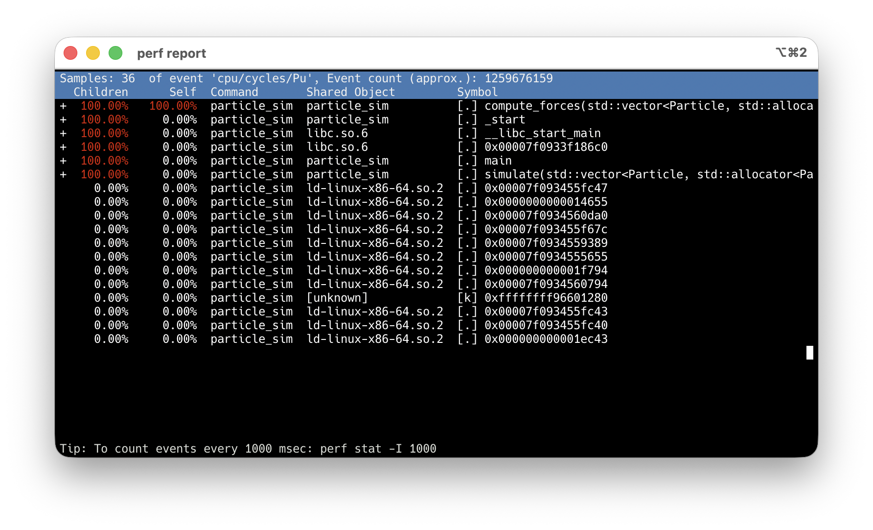
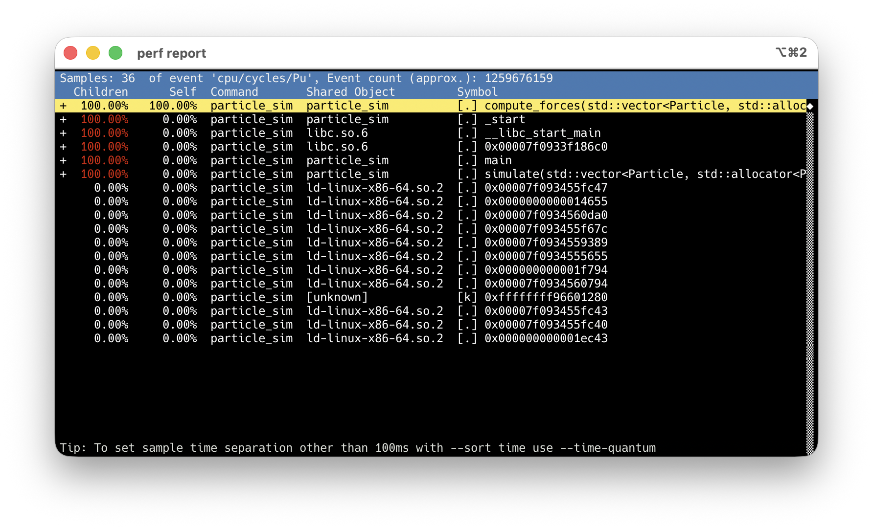
-O2 -g: debug info maps samples to source lines. Never use -O0.

compute_forces at 100% Children — every sample goes through it.

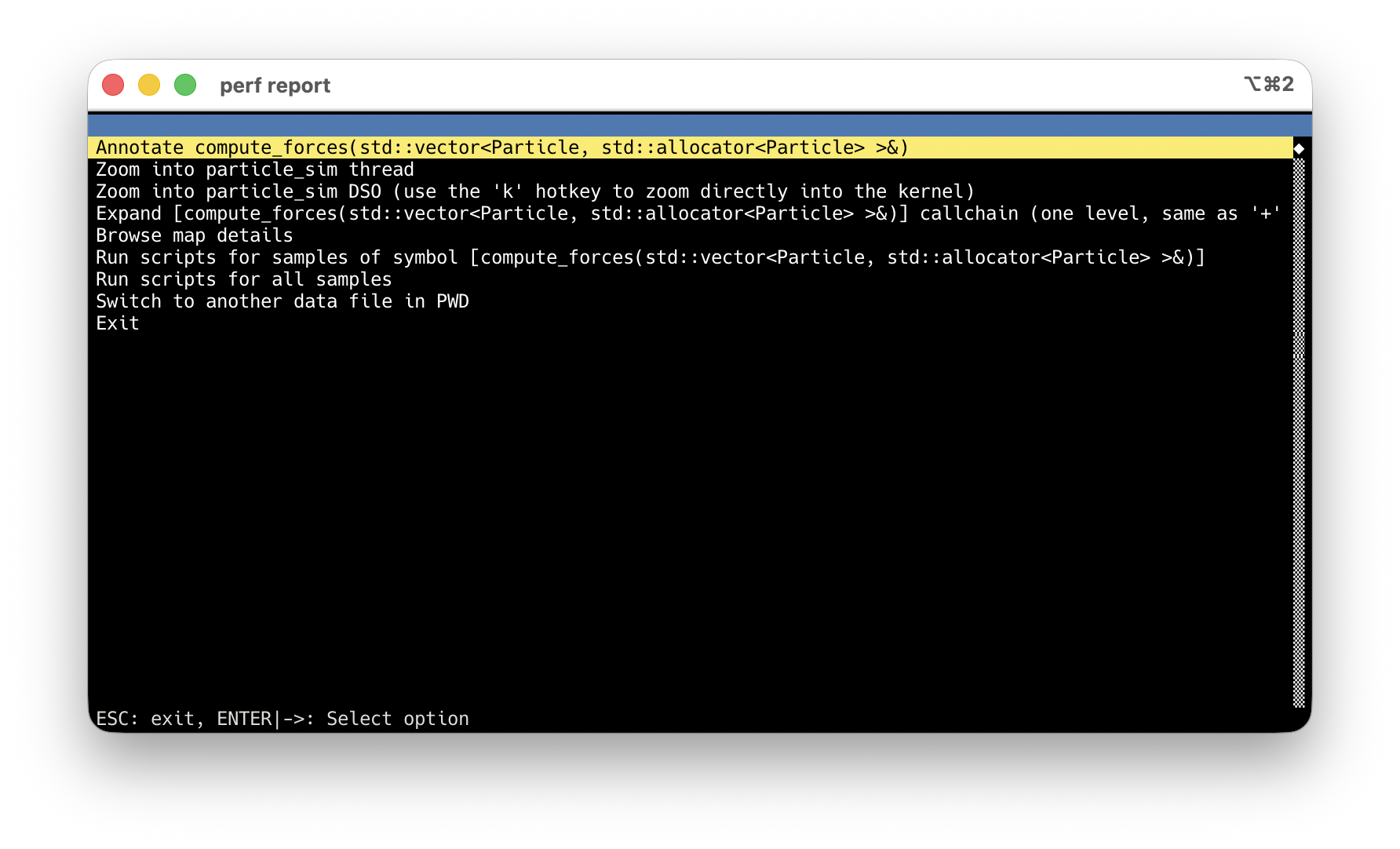
Arrow keys → highlight the hot symbol.

Enter → action menu → Annotate.

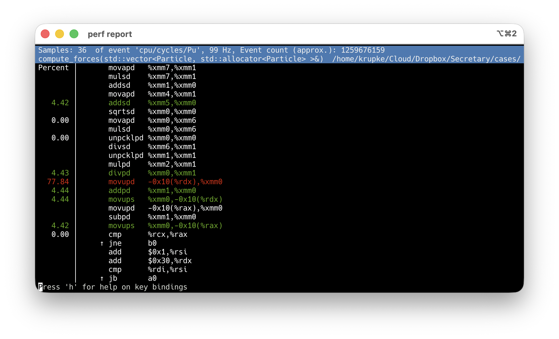
Default: asm-only, sample % per instruction.

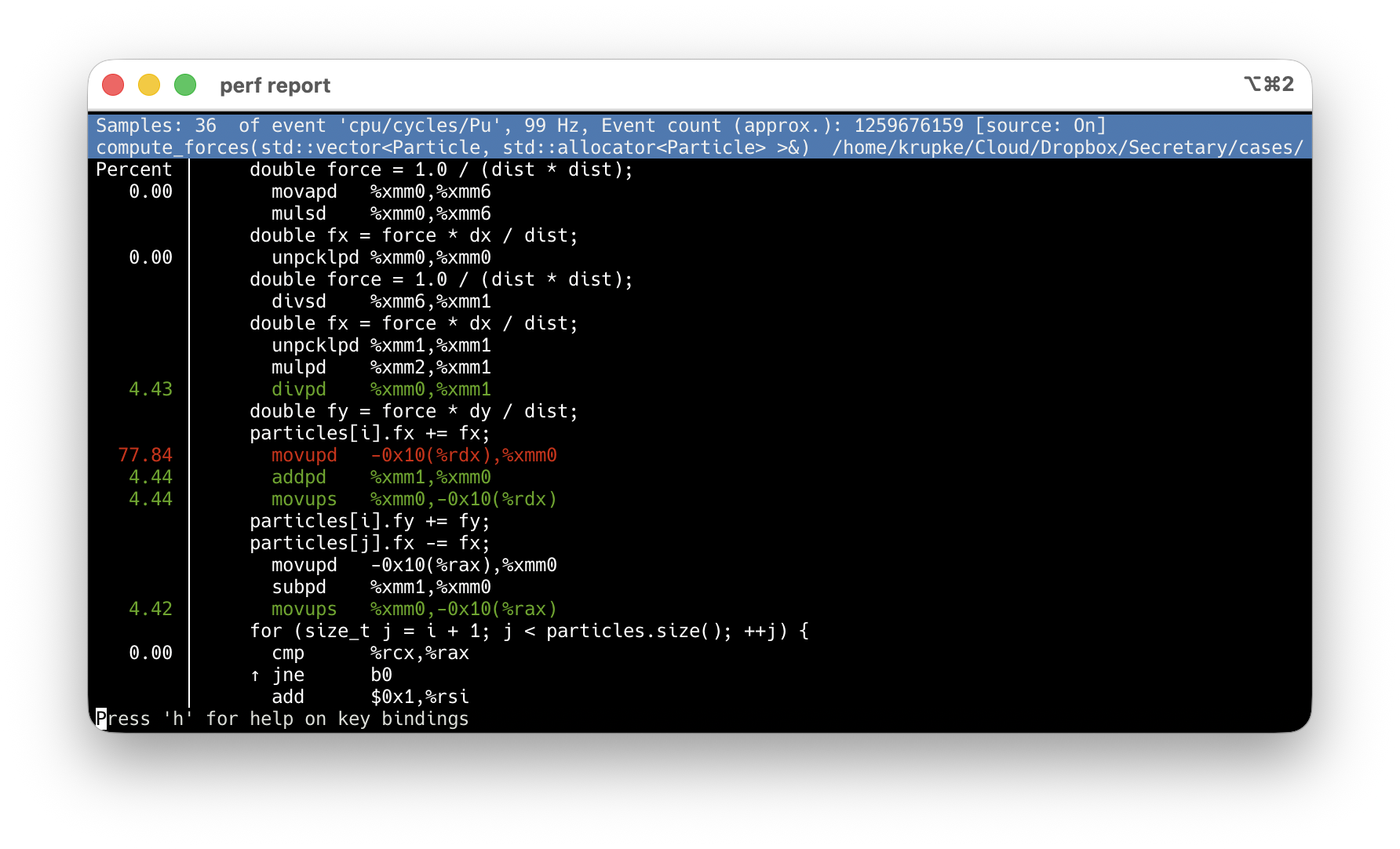
Press s → source interleaved. Inlined code too.

Micro-benchmarking

Profiling finds where the bottleneck is. Micro-benchmarking measures whether your fix actually helped.

Python: `timeit` — Basic Usage (wall-clock time)

import timeit

n = 100_000
t_comp = timeit.timeit(  # returns total seconds for `number` runs
    lambda: [x**2 for x in range(n)], number=50
)
t_map = timeit.timeit(
    lambda: list(map(lambda x: x**2, range(n))), number=50
)
print(f"comprehension: {t_comp:.3f}s   map: {t_map:.3f}s   ratio: {t_comp/t_map:.2f}x")

comprehension: 2.261s   map: 3.307s   ratio: 0.68x

C++: Google Benchmark — Our Example

We benchmark two graph representations with the same API:

Which layout is faster for graph traversal at scale?

C++: Google Benchmark — Writing a Benchmark

static void BM_iterate_neighbors_csr(benchmark::State& state) {
    int n = static_cast<int>(state.range(0));  // parameter from Range()
    auto edges = random_edges(n, num_edges(n));
    auto graph = make_csr(n, edges);           // setup: NOT measured

    for (auto _ : state) {                     // measured loop
        long sum = 0;
        for (int v = 0; v < graph.num_vertices(); v++) {
            for (int u : graph.neighbors(v)) sum += u;
        }
        benchmark::DoNotOptimize(sum);         // prevent dead-code elimination
    }
    state.SetItemsProcessed(state.iterations() * graph.num_edges() * 2);
}
BENCHMARK(BM_iterate_neighbors_csr)->RangeMultiplier(10)->Range(1000, 1000000);

Concept	What it does
Setup before loop	Excluded from timing
`for (auto _ : state)`	Framework controls iteration count
`DoNotOptimize(val)`	Prevents compiler from eliminating unused results
`SetItemsProcessed`	Enables throughput reporting (items/s)
`Range(lo, hi)`	Sweeps input sizes automatically

Google Benchmark: Example Output

Benchmark                                      Time        CPU   UserCounters
BM_iterate_neighbors_adjlist/1000          1,469 ns    1,465 ns   6.82G items/s
BM_iterate_neighbors_csr/1000              1,475 ns    1,472 ns   6.79G items/s
BM_iterate_neighbors_adjlist/1000000   14,541,591 ns  14,497 us   690M items/s
BM_iterate_neighbors_csr/1000000        8,369,209 ns   8,347 us   1.20G items/s

At N=1000: both fit in cache — no difference. At N=1M: CSR is 1.7x faster — memory layout matters.

Same semantics, different memory behavior — exactly the kind of result microbenchmarks should explain.

We have a plausible explanation — but perf stat can turn it into evidence.

Source: examples/google_benchmark/ — you will get this template.

Benchmark + `perf stat`: Why Is CSR Faster?

Filter to one case, wrap the binary with perf stat:

perf stat -r 3 -e cycles,instructions,cache-references,cache-misses \
  ./bm_graph --benchmark_filter='BM_iterate_neighbors_adjlist/1000000$' \
             --benchmark_min_time=2s
# repeat with …_csr/1000000$

Counter (per iteration)	adjlist	CSR	Ratio
time	13.76 ms	8.39 ms	1.64× faster
instructions / cycle	0.29	0.37	1.26×
L1-dcache miss rate	8.1%	5.6%	—
cache-misses (≈ DRAM)	5.02 M	1.80 M	2.79× fewer

Benchmark tells you how much. perf stat tells you why. Roughly 2.8× fewer DRAM-class misses — the pipeline is no longer starved.

Use the generic cache-references / cache-misses events — LLC-loads / LLC-load-misses report <not supported> on AMD Zen.

Setting Up Google Benchmark: Project Layout

my_project/
├── CMakeLists.txt              # root: fetch deps, add subdirectories
├── src/
│   ├── CMakeLists.txt          # defines the library target
│   └── graph/
│       ├── graph.h             # your library headers
│       └── graph_gen.h
├── benchmarks/
│   ├── CMakeLists.txt          # benchmark targets, link against library
│   └── bm_graph.cpp
└── tests/
    ├── CMakeLists.txt          # test targets, link against library
    └── test_graph.cpp

src/ defines a library target. Benchmarks and tests both link against it — same include paths, same compile settings, no relative-path #include hacks.

Setting Up: Root `CMakeLists.txt`

cmake_minimum_required(VERSION 3.14)
project(my_project LANGUAGES CXX)
include(FetchContent)     # downloads libraries as part of cmake build

# Google Benchmark — fetched automatically, no manual install
FetchContent_Declare(googlebenchmark
    GIT_REPOSITORY https://github.com/google/benchmark.git
    GIT_TAG        v1.9.4)

# Don't build benchmark's own tests (we don't need them)
set(BENCHMARK_ENABLE_TESTING OFF CACHE BOOL "" FORCE)
set(BENCHMARK_ENABLE_INSTALL OFF CACHE BOOL "" FORCE)
FetchContent_MakeAvailable(googlebenchmark)

add_subdirectory(src)          # your library (INTERFACE target)
add_subdirectory(tests)
add_subdirectory(benchmarks)

FetchContent downloads + builds Google Benchmark automatically. Just run cmake — no system-wide installation needed.

Full example with Google Test: examples/google_benchmark/CMakeLists.txt

Setting Up: `benchmarks/CMakeLists.txt`

add_executable(bm_my_algorithm bm_my_algorithm.cpp)

# Link against your library and Google Benchmark.
# my_lib provides include paths + compile settings (e.g., C++20).
# benchmark_main provides main() with built-in CLI flag parsing.
target_link_libraries(bm_my_algorithm my_lib benchmark::benchmark_main)

Build and run:

cmake -B build -DCMAKE_BUILD_TYPE=Release    # Release is critical!
cmake --build build
./build/benchmarks/bm_my_algorithm

Warning

Always use CMAKE_BUILD_TYPE=Release. Debug mode uses -O0 (no optimization) — your benchmarks will measure unoptimized code and the results are meaningless.

Full example: examples/google_benchmark/benchmarks/CMakeLists.txt — your existing src/ and tests/ stay untouched; benchmarks are additive.

Google Benchmark: Useful Flags

# Run only benchmarks matching a regex
./build/benchmarks/bm_graph --benchmark_filter=BFS

# JSON output for scripts/plotting
./build/benchmarks/bm_graph --benchmark_format=json \
                             --benchmark_out=results.json

# Multiple repetitions → mean, median, stddev
./build/benchmarks/bm_graph --benchmark_repetitions=5

# Combine: filter + repetitions + save to file
./build/benchmarks/bm_graph --benchmark_filter=iterate \
                             --benchmark_repetitions=5 \
                             --benchmark_format=json \
                             --benchmark_out=results.json

All flags are built into benchmark_main — no code changes needed.

Block 2: Achieve Performance

Now we know where the time goes. Here’s how to make it faster — in Python and in C++.

Python Performance Killers

Common patterns that are silently expensive. Each one is easy to fix — once you know it’s there.

`x in list` is secretly O(n)

Slow:

users = list(range(10_000))
count = 0
for q in queries:
    if q in users:       # linear scan!
        count += 1

Fast:

users = set(range(10_000))
count = 0
for q in queries:
    if q in users:       # hash lookup
        count += 1

list: 128.6 ms   set: 0.12 ms   speedup: 1034x

Building a temporary data structure just for faster lookups may feel redundant — but it is often the single most effective optimization.

Detour: `std::set` vs `std::vector` — not like Python

In Python, set always beats list for lookups (1000x). In C++, the picture is very different.

100k lookups against a container of size N:

N	unsorted `vector` O(n)	`std::set` O(log n)	sorted `vector` O(log n)
1K	1.5 ms	1.9 ms	1.7 ms
10K	126 ms	4.2 ms	2.4 ms
100K	1,258 ms	11.9 ms	3.5 ms
1M	12,690 ms	29.2 ms	4.9 ms

At N=10K, std::set beats the linear scan by only 30x — not 1000x like in Python. And the sorted vector beats std::set by up to 6x — same O(log n), fewer cache misses.

In C++, data layout often matters more than algorithmic complexity class. Prefer flat, contiguous containers unless insertions/deletions at scale make re-sorting too expensive.

String concatenation in loops

Slow:

s = ""
for part in parts:
    s += part         # new string each time

Fast:

s = "".join(parts)    # one allocation

s += part:     2.63 ms
"".join():     0.14 ms     speedup: 18x

Strings are immutable in Python. Each += copies the entire string so far. That is \(O(n^2)\) in total length.

Use builtins instead of manual loops

Slow:

total = 0
for x in xs:
    total += x

Fast:

total = sum(xs)

manual loop: 7.21 ms     sum(): 1.87 ms     speedup: 3.9x

Also applies to min(), max(), any(), all() — all run in C, not Python bytecode.

The general principle: push hot iterations into C-level code paths — the same idea as pybind11, just within the standard library.

Memoization with `@lru_cache`

Slow:

def fib(n):
    if n < 2: return n
    return fib(n-1) + fib(n-2)

Fast:

from functools import lru_cache

@lru_cache(maxsize=None)
def fib(n):
    if n < 2: return n
    return fib(n-1) + fib(n-2)

fib(32) naive:   390 ms
fib(32) cached:  0.008 ms     speedup: 50,000x

Python’s @lru_cache makes this a one-line fix. Any pure function with repeated inputs is a candidate — DP subproblems, normalization, parsing.

Push numeric work to NumPy

Slow:

# Python nested loops
for i in range(n):
    for k in range(n):
        for j in range(n):
            C[i][j] += A[i][k] * B[k][j]

Fast:

import numpy as np

C = A @ B    # delegates to BLAS

Python loops (200x200): 436 ms
NumPy A @ B (200x200):  0.087 ms     speedup: 5000x

If Scalene shows high Python time on numeric loops, NumPy (or moving to C++) is the answer — not micro-optimizing the loop.

Data containers: cost of abstraction

Creating 100k objects with three float fields:

Container	Creation	Create + access	Relative
`tuple`	1.0 ms	11 ms	1x
`class` / `dataclass`	15 ms	23 ms	~2x
`dataclass(slots=True)`	14 ms	22 ms	~2x
`NamedTuple`	18 ms	27 ms	~2.4x
Pydantic `BaseModel`	51 ms	59 ms	~5x

Pydantic validates and coerces every field on every instantiation. That is invaluable at system boundaries — and ruinous in a hot loop.

Use Pydantic for parsing external input (API, config, files). Use dataclass(slots=True) or plain tuples for internal data that gets created millions of times.

Moving to Native: pybind11

The bottleneck is not “Python”. The bottleneck is the interpreted loop.

When pybind11 is worth it

Scalene shows most time in Python execution
the hotspot is a tight inner loop
the Python-side implementation is fundamentally loop-heavy
moving the whole loop is realistic

Our example: TSP nearest-neighbor + 2-opt local search. Both are tight O(n²) loops over distance computations — exactly the pattern where moving the entire loop to C++ pays off.

If the bottleneck is CPU-bound — especially superlinear algorithms — copying data into C++ and back is often worth it. The copy cost is linear; the savings are superlinear.

The measured difference

TSP benchmark, N = 1000

Python:
  Nearest neighbor:  0.059s
  2-opt:             1.259s
  Total:             1.318s

C++ (on-the-fly):
  Nearest neighbor:  0.001s
  2-opt:             0.007s
  Total:             0.007s

C++ (precomputed):
  Total:             0.005s

Tour quality: identical

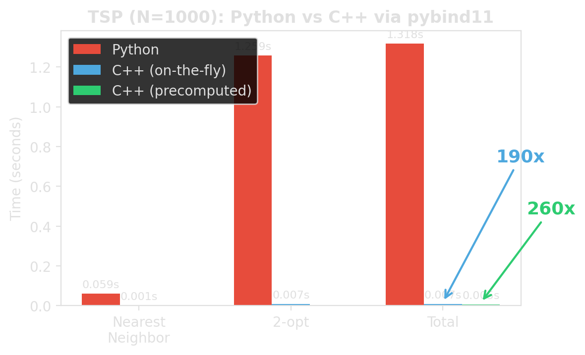
Same algorithm. Same result. Roughly 190x / 260x faster. Different place where the loop runs.

Source: examples/pybind11_template/benchmark_python_vs_cpp.py

The workflow

Write the algorithm in pure C++ — no pybind11 dependency
Write a thin binding file — converts Python types to C++ and back
Configure the build — pyproject.toml + CMakeLists.txt
Install with pip — pip install -e . builds everything
Import from Python — import fast_tsp; fast_tsp.nearest_neighbor(cities)

my_package/
├── pyproject.toml              # build config (scikit-build-core + pybind11)
├── CMakeLists.txt              # compile the C++ extension
├── src/my_package/
│   ├── algorithm.h / .cpp      # pure C++ (no pybind11 dependency)
│   ├── _bindings.cpp           # thin pybind11 wrapper
│   └── __init__.py             # re-export C++ functions
└── tests/

Step 1: Write the C++ algorithm

// tsp.h — pure C++, no pybind11 dependency
struct Point {
    double x;
    double y;
};

inline double dist(const Point& a, const Point& b) {
    double dx = a.x - b.x;
    double dy = a.y - b.y;
    return std::sqrt(dx * dx + dy * dy);
}

std::vector<int> two_opt_improve(std::span<const Point> cities,
                                  std::vector<int> tour) {
    int n = static_cast<int>(tour.size());
    bool improved = true;
    while (improved) {
        improved = false;
        for (int i = 0; i < n - 1; i++) {
            for (int j = i + 2; j < n; j++) {
                double old_d = dist(cities[tour[i]], cities[tour[i+1]])
                             + dist(cities[tour[j]], cities[tour[(j+1)%n]]);
                double new_d = dist(cities[tour[i]], cities[tour[j]])
                             + dist(cities[tour[i+1]], cities[tour[(j+1)%n]]);
                if (new_d < old_d - 1e-10) {
                    std::reverse(tour.begin()+i+1, tour.begin()+j+1);
                    improved = true;
                }
            }
        }
    }
    return tour;
}

Full code: examples/pybind11_template/src/fast_tsp/tsp.h

Step 2: Write the binding file

#include <pybind11/pybind11.h>
#include <pybind11/stl.h>       // auto-convert std::vector <-> Python list
#include <array>
#include "tsp.h"
namespace py = pybind11;

PYBIND11_MODULE(_native, m) {
    m.doc() = "fast_tsp C++ extension — TSP routines via pybind11";

    m.def("nearest_neighbor",
          [](const std::vector<std::array<double, 2>>& cities) {
              std::vector<Point> pts; pts.reserve(cities.size());
              for (auto& c : cities) pts.push_back({c[0], c[1]});
              py::gil_scoped_release release;    // let other Python threads run
              return nearest_neighbor(pts);      // std::vector<int> → list
          },
          "Nearest neighbor heuristic",
          py::arg("cities"));

    m.def("two_opt_improve",
          [](const std::vector<std::array<double, 2>>& cities,
             std::vector<int> tour) {
              std::vector<Point> pts; pts.reserve(cities.size());
              for (auto& c : cities) pts.push_back({c[0], c[1]});
              py::gil_scoped_release release;
              return two_opt_improve(pts, std::move(tour));
          },
          py::arg("cities"), py::arg("tour"));

    // Precomputed distance matrix for repeated access (e.g., multi-pass 2-opt)
    py::class_<DistanceMatrix>(m, "DistanceMatrix")
        .def(py::init([](const std::vector<std::array<double, 2>>& cities) {
                 std::vector<Point> pts; pts.reserve(cities.size());
                 for (auto& c : cities) pts.push_back({c[0], c[1]});
                 return DistanceMatrix(pts);
             }),
             py::arg("cities"))
        .def_property_readonly("size", &DistanceMatrix::size)
        .def("query", &DistanceMatrix::operator(),
             py::arg("i"), py::arg("j"));

    // Overloads taking DistanceMatrix instead of coordinates
    m.def("two_opt_improve",
          [](const DistanceMatrix& dm, std::vector<int> tour) {
              py::gil_scoped_release release;
              return two_opt_improve(dm, std::move(tour));
          },
          py::arg("distances"), py::arg("tour"));

    m.def("nearest_neighbor",
          [](const DistanceMatrix& dm) {
              py::gil_scoped_release release;
              return nearest_neighbor(dm);
          },
          py::arg("distances"));
}

Source: examples/pybind11_template/src/fast_tsp/_bindings.cpp

Step 3: `pyproject.toml` + `CMakeLists.txt`

The build config has two pybind11-specific parts:

pyproject.toml — build system:

[build-system]
requires = [
  "scikit-build-core>=0.12.2",
  "pybind11>=3.0.3"
]
build-backend = "scikit_build_core.build"

[tool.scikit-build]
wheel.packages = ["src/fast_tsp"]

[tool.scikit-build.cmake]
build-type = "Release"

CMakeLists.txt — compile the extension:

cmake_minimum_required(VERSION 3.15...3.30)
project(${SKBUILD_PROJECT_NAME} LANGUAGES CXX)

set(PYBIND11_FINDPYTHON ON)
find_package(pybind11 3.0 CONFIG REQUIRED)

pybind11_add_module(_native
    src/fast_tsp/tsp.cpp
    src/fast_tsp/_bindings.cpp)

target_compile_features(_native PRIVATE cxx_std_20)
install(TARGETS _native DESTINATION fast_tsp)

pip install -e . calls scikit-build-core, which calls CMake, which compiles the extension. The rest of pyproject.toml ([project] name, version, dependencies) is standard Python packaging.

Full files: examples/pybind11_template/pyproject.toml, CMakeLists.txt

Step 4: `init.py` and install

# src/fast_tsp/__init__.py — re-export C++ functions
from fast_tsp._native import nearest_neighbor, two_opt_improve, tour_length

Build and install:

pip install -e ".[test]"      # editable install + test deps

Use from Python:

import fast_tsp

cities = [(0.0, 0.0), (1.0, 0.0), (1.0, 1.0), (0.0, 1.0)]
tour = fast_tsp.nearest_neighbor(cities)           # → list[int]
tour = fast_tsp.two_opt_improve(cities, tour)      # → list[int]
print(f"Tour length: {fast_tsp.tour_length(cities, tour):.1f}")

Full template: examples/pybind11_template/

Distributing compiled extensions

pip install -e . works locally — but requires a C++ compiler + CMake on the target
Extensions are bound to a specific Python version and platform
Wheels are pre-compiled — pip install just unpacks, no build tools needed
cibuildwheel + GitHub Actions automates building wheels for all platforms

For course projects, editable installs are fine. For packages you share, build wheels in CI so users never need a compiler.

C++ Performance Killers

Now the bottleneck is inside C++. Same principle: measure, then fix the right thing.

Accidental copies: `auto r` vs `const auto& r`

Slow:

struct Record { std::vector<int> payload; };

size_t total(const std::vector<Record>& rs) {
    size_t sum = 0;
    for (auto r : rs)            // copies!
        sum += r.payload.size();
    return sum;
}

Fast:

struct Record { std::vector<int> payload; };

size_t total(const std::vector<Record>& rs) {
    size_t sum = 0;
    for (const auto& r : rs)    // no copy
        sum += r.payload.size();
    return sum;
}

100k records x 32 ints:
  auto r (copy):       51.9 ms
  const auto& r (ref):  2.4 ms     speedup: 21x

One character (&) eliminates 100,000 heap allocations per iteration.

Missing `reserve()` for `push_back`

Slow:

std::vector<int> build(size_t n) {
    std::vector<int> v;
    for (size_t i = 0; i < n; ++i)
        v.push_back(i);
    return v;
}

Fast:

std::vector<int> build(size_t n) {
    std::vector<int> v;
    v.reserve(n);
    for (size_t i = 0; i < n; ++i)
        v.push_back(i);
    return v;
}

10M push_backs:
  no reserve():    210 ms
  with reserve():   87 ms     speedup: 2.4x

Without reserve, the vector reallocates and copies ~24 times for 10M elements. Each reallocation touches an ever-larger memory region, thrashing the cache.

Erase-in-loop: O(n^2) hiding in plain sight

Slow:

void remove_negatives(std::vector<int>& v) {
    for (auto it = v.begin(); it != v.end();) {
        if (*it < 0)
            it = v.erase(it);  // shifts tail
        else
            ++it;
    }
}

Fast:

void remove_negatives(std::vector<int>& v) {
    v.erase(
        std::remove_if(v.begin(), v.end(),
            [](int x) { return x < 0; }),
        v.end());
}

200k elements, ~33% removed:
  erase in loop:   132 ms
  erase-remove:    0.38 ms     speedup: 344x

Each erase() shifts all following elements. Repeated erases: \(\sum_{k=1}^{n} O(n-k) = O(n^2)\).

Memory layout: AoS vs SoA

AoS (Array of Structs):

struct Particle {  // 32 bytes
    float x, y, z;
    float vx, vy, vz;
    uint32_t id, flags;
};

float sum_x(const std::vector<Particle>& ps) {
    float s = 0;
    for (const auto& p : ps) s += p.x;
    return s;
}

SoA (Struct of Arrays):

struct ParticlesSoA {
    std::vector<float> x, y, z;
    std::vector<float> vx, vy, vz;
};

float sum_x(const ParticlesSoA& ps) {
    float s = 0;
    for (float xi : ps.x) s += xi;
    return s;
}

10M particles, sum one field:
  AoS (32B stride): 342 ms
  SoA (4B stride):  181 ms     speedup: 1.9x

AoS reads 32 bytes per element but uses only 4. 7/8 of cache bandwidth is wasted.

Why AoS wastes cache bandwidth

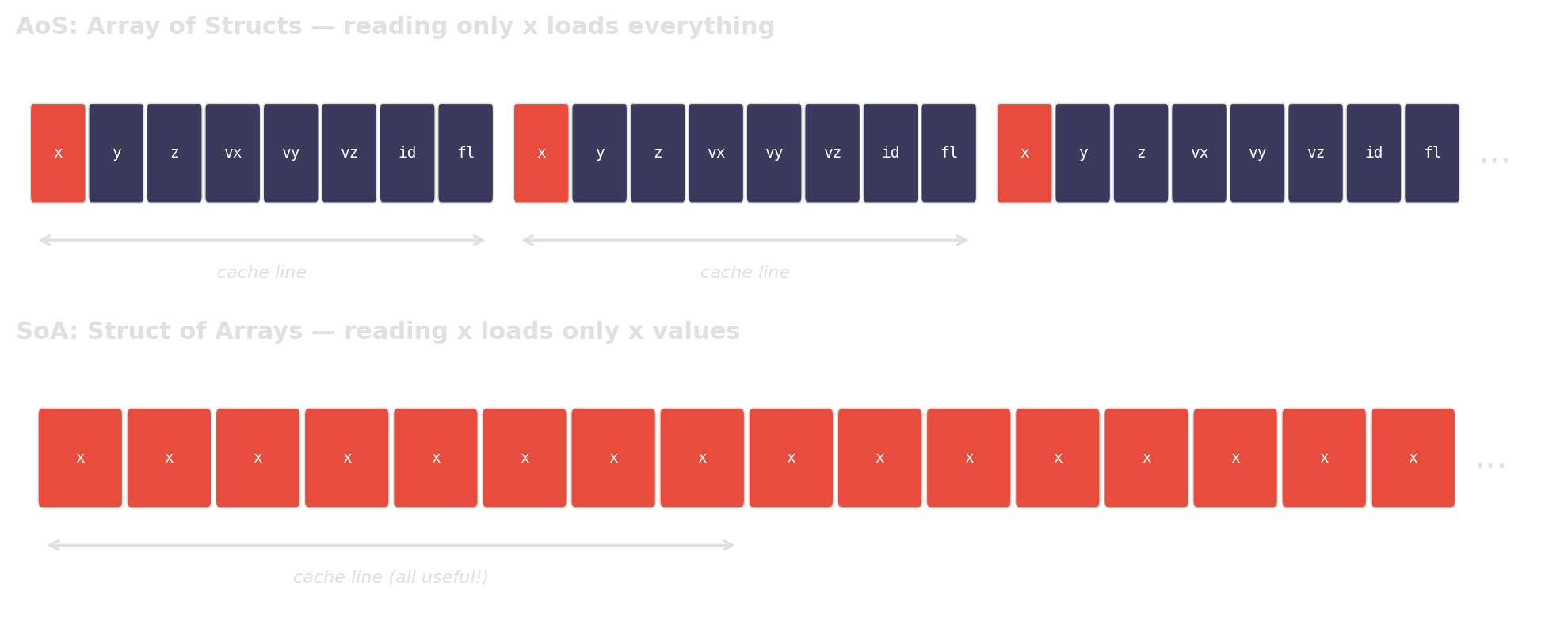
When you only access one field, AoS forces the CPU to load the entire struct per element. SoA packs the relevant data contiguously, so every cache line is fully utilized.

Pointer chasing: `std::list` vs `std::vector`

Slow:

// linked list: each node is a separate
// heap allocation → pointer chase
std::list<int> data;
for (int i = 0; i < N; i++)
    data.push_back(i);

long sum = 0;
for (int x : data) sum += x;  // cache miss per node

Fast:

// vector: contiguous memory
// → hardware prefetcher streams it
std::vector<int> data(N);
std::iota(data.begin(), data.end(), 0);

long sum = 0;
for (int x : data) sum += x;  // sequential scan

1M elements, sum all values:
  std::list (sequential alloc):    1.1 ms     29x slower
  std::list (shuffled / realistic):  58 ms     1500x slower
  std::vector (contiguous):       0.04 ms     baseline

Sequentially allocated nodes happen to sit nearby in memory — best case. In real programs, nodes are interleaved with other allocations — worst case.

Every node->next is a potential cache miss. A flat array lets the prefetcher do its job.

Accidental \(O(n^2)\): dedup with nested loops

Slow:

std::vector<int> dedup(const std::vector<int>& in) {
    std::vector<int> out;
    for (int x : in) {
        bool seen = false;
        for (int y : out)   // linear scan!
            if (y == x) { seen = true; break; }
        if (!seen) out.push_back(x);
    }
    return out;
}

Fast:

std::vector<int> dedup(std::vector<int> v) {
    std::sort(v.begin(), v.end());
    v.erase(
        std::unique(v.begin(), v.end()),
        v.end());
    return v;
}

100k integers:
  nested loop O(n²):     349 ms
  sort + unique O(n log n): 3.9 ms     speedup: 89x

Algorithmic thinking is not just for Python. The same complexity traps appear in C++ — the fix is often a standard-library one-liner.

Wrap-up

The discipline matters more than the specific tools.

Same discipline, every time

Find the dominant cost — logging, then profilers
Classify the bottleneck — algorithmic? interpreter overhead? memory layout?
Change one thing — the thing the evidence points to
Verify on the same workload — timeit, Google Benchmark, or just timestamps

pybind11 is not “make it fast”. Google Benchmark is not “time it nicely”. Both are part of a measurement-driven workflow.

Concepts, not tools

Tool	Concept	Alternatives
`logging`	Structured observability	`loguru`, `spdlog` (C++)
Scalene	Sampling profiler (Python)	`py-spy`, VTune
`perf`	Sampling profiler (C++)	VTune, `Instruments` (macOS)
cProfile	Tracing profiler	`yappi`, `gprof`
pybind11	Native bindings for Python	`nanobind`, `cython`, `PyO3`
`timeit`	Microbenchmarking (Python)	`pytest-benchmark`
Google Benchmark	Microbenchmarking (C++)	`Catch2`, `criterion` (Rust)

Links

C++ Core Guidelines	Parameter passing, copy semantics, best practices
Google Benchmark	Microbenchmarking framework for C++
pybind11 Documentation	C++/Python bindings — reference & tutorial
Course Material Repository	Slides, examples, and exercises

References

Knuth, Donald E. 1974. “Structured Programming with Go to Statements.” ACM Comput. Surv. (New York, NY, USA) 6 (4): 261–301. https://doi.org/10.1145/356635.356640.

Performance Engineering in Practice

Performance Engineering in Practice

Block 1: Find the Bottleneck

Amdahl’s law: know the ceiling

“Premature optimization is the root of all evil”

Observability: Basic Logging

Start with phase markers

What the timestamps reveal

Add structural context

Controlling verbosity per component

Guard expensive log computations

Good code has logging — especially in production

Profiling

Two big families

What does “time” even mean?

A practical rule of thumb

cProfile: when you want exact call counts

cProfile: targeted profiling

Scalene: when you want line-level insight (wall-clock, Python/native split)

Reading Scalene output

C++ profiling with perf

perf answers two questions

perf stat — classify

Read the signature, not the number

perf record + perf report: find the hotspot

Micro-benchmarking

Python: timeit — Basic Usage (wall-clock time)

C++: Google Benchmark — Our Example

C++: Google Benchmark — Writing a Benchmark

Google Benchmark: Example Output

Benchmark + perf stat: Why Is CSR Faster?

Setting Up Google Benchmark: Project Layout

Setting Up: Root CMakeLists.txt

Setting Up: benchmarks/CMakeLists.txt

Google Benchmark: Useful Flags

Block 2: Achieve Performance

Python Performance Killers

x in list is secretly O(n)

Detour: std::set vs std::vector — not like Python

String concatenation in loops

Use builtins instead of manual loops

Memoization with @lru_cache

Push numeric work to NumPy

Data containers: cost of abstraction

Moving to Native: pybind11

When pybind11 is worth it

The measured difference

The workflow

Step 1: Write the C++ algorithm

Step 2: Write the binding file

Step 3: pyproject.toml + CMakeLists.txt

Step 4: __init__.py and install

Distributing compiled extensions

C++ Performance Killers

Accidental copies: auto r vs const auto& r

Missing reserve() for push_back

Erase-in-loop: O(n^2) hiding in plain sight

Memory layout: AoS vs SoA

Why AoS wastes cache bandwidth

Pointer chasing: std::list vs std::vector

Accidental \(O(n^2)\): dedup with nested loops

Wrap-up

Same discipline, every time

Concepts, not tools

Further reading

Links

References

C++ profiling with `perf`

`perf` answers two questions

`perf stat` — classify

`perf record` + `perf report`: find the hotspot

Python: `timeit` — Basic Usage (wall-clock time)

Benchmark + `perf stat`: Why Is CSR Faster?

Setting Up: Root `CMakeLists.txt`

Setting Up: `benchmarks/CMakeLists.txt`

`x in list` is secretly O(n)

Detour: `std::set` vs `std::vector` — not like Python

Memoization with `@lru_cache`

Step 3: `pyproject.toml` + `CMakeLists.txt`

Step 4: `init.py` and install

Accidental copies: `auto r` vs `const auto& r`

Missing `reserve()` for `push_back`

Pointer chasing: `std::list` vs `std::vector`

References

Algorithm Engineering SS 2026 — T01 Performance Engineering