LP/MIP Modeling

Algorithm Engineering — T03
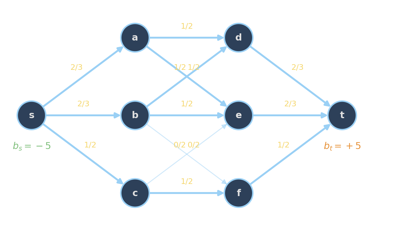
Dr. Dominik Krupke

Welcome

LP/MIP Modeling

Two Problem Classes with Powerful Solvers

Linear Expressions

\[ \begin{aligned} \max\quad & \sum_{e \in \delta^+(s)} x_e \\ \text{s.t.}\quad & \sum_{e \in \delta^+(v)} x_e = \sum_{e \in \delta^-(v)} x_e & \forall v \in V \\ & 0 \le x_e \le u_e & \forall e \in E \end{aligned} \]

\[ \begin{aligned} \max\quad & \sum_i v_i\, b_i \\ \text{s.t.}\quad & \sum_i w_i\, b_i \le W \\ & b_i \in \{0, 1\} && \forall i \end{aligned} \]

Continuous Variables (Linear Programs)

Solvable in polynomial time.

Discrete Variables (Mixed-Integer Programs)

NP-hard in general but often tractable.

For both problem classes, there are highly engineered solvers. How much can we express in each class? How do we know if it is the right technology?

The diet problem

\[ \begin{aligned} \min\quad & \sum_j c_j\, x_j \\ \text{s.t.}\quad & \sum_j a_{ij}\, x_j \;\ge\; b_i & \forall i \\ & x_j \ge 0 \end{aligned} \]

Choose food quantities \(x_j\) to meet every nutrient requirement \(b_i\) at minimum cost. Coefficient \(a_{ij}\) = nutrient \(i\) per unit of food \(j\).

Food \(j\) kcal protein (g) calcium (mg) \(c_j\) (€/unit)
Oats 380 13 50 0.20
Milk 150 8 300 0.80
Eggs 80 7 30 0.30
Beans 230 15 80 0.40
Daily req. \(b_i\) 2000 50 800

Real-world siblings:

  • Feed formulation: livestock rations from grains
  • Alloy blending: composition spec from raw metals
  • Fuel mix: octane rating from crude streams
  • Fertilizer mixing: N/P/K from base products
  • Production mix: products from limited resources

Network Flow

\[ \min\quad \sum_{e \in E} c_e\, x_e \] \[ \sum_{e \in \delta^-(v)} x_e - \sum_{e \in \delta^+(v)} x_e = b_v\quad \forall v \in V \\ 0 \le x_e \le u_e \quad \forall e \in E \]

Real-world siblings:

  • Shipping & logistics: origins to destinations
  • Telecom routing: link capacities, endpoint demand
  • Power dispatch: generation, load, transmission
  • Supply chains: multi-stage production
  • Pipeline scheduling: capacitated arcs

Special cases: shortest path, max-flow, transportation, assignment.


Edge labels: flow \(x_e\) / capacity \(u_e\). \(b_v < 0\) supplies, \(b_v > 0\) demands.

Matchings/Assignments

\[ \begin{aligned} \max\quad & \sum_{e \in E} c_e\, x_e \\ \text{s.t.}\quad & \sum_{e \in \delta(v)} x_e \;\le\; 1 && \forall v \in V \\ & x_e \in \{0,1\} \end{aligned} \]

Pick edges of an undirected graph to maximize total weight, no two chosen edges sharing a vertex. A vertex may stay unmatched.

Real-world siblings:

  • Roommate pairing: dorm allocation
  • Tournament rounds: chess Swiss-style pairings
  • Ride-share pairing: two riders share a car
  • Kidney exchange: donor-recipient pairs
  • Peer programming: students paired by skill

The basic version is polynomial, but as soon as there are interdependencies between edges or we have t-wise instead of pairwise matchings, the Blossom algorithm fails and we need MIP.

Set Cover

\[ \begin{aligned} \min\quad & \sum_{S \in \mathcal{S}} c_S\, y_S \\ \text{s.t.}\quad & \sum_{S \ni i} y_S \;\ge\; 1 && \forall\ i\\ & y_S \in \{0,1\} \end{aligned} \]

Pick subsets \(S\) so every element \(i\) is covered at least once, at minimum cost.

Real-world siblings:

  • Crew scheduling: duty patterns covering all flights
  • Facility location: depots covering all customer regions
  • Survey routing: routes covering all neighborhoods
  • Sensor placement: cameras covering all zones
  • Vaccine outreach: clinics covering all populations

Surprisingly many difficult combinatorial optimization problems turn out to be variants of Set Cover (\(\geq 1\)), Set Packing (\(\leq 1\)), or Set Partitioning (\(=1\)) at heart.

But what if my problem has non-linear expressions?

# Expression \(\mathrel{\hat{=}}\text{LP}\) \(\mathrel{\hat{=}}\text{MIP}\) approx. only
1 \(\min\ \max_i\, c_i^\top x_i, x\in \mathbb{R}^n\)
2 \(\max\ \sum_i \lvert x_i \rvert, x\in \mathbb{R}^n\)
3 \(\min\ \sum_i \lvert x_i \rvert, x\in \mathbb{R}^n\)
4 \(\min\ \sum_i x_i^2, x\in \mathbb{R}^n\)
5 \(c^\top x \ge a\ \ \lor\ \ c'^\top x \le a', x\in \mathbb{R}^n\)
6 \(z = x\,y,\ x \in \{0,1\},\ y \in [L, U]\)
7 \(z = x\,y,\ x, y \in [L, U]\)

Things are not always as they seem. Which of these non-linear expressions are actually linear in disguise?

“All models are wrong, but some are useful.” (George Box)

  • Modeling is a constant tension between accuracy and tractability.
  • LPs are one of the most benign (optimization) problem classes available.
    • Highly optimized solvers solving millions of variables in seconds.
  • Well-formulated MIPs are also often quite tractable.
    • In particular, if the LP relaxation is tight.
  • Detecting tractable modeling patterns is the critical skill for building useful models.

“Every hard problem has a weakness. The modeler’s art is to find it before the solver finds despair.”

— Confucypus

Speaking to the solver

Once you know the basics, you can essentially use any LP/MIP solver you like.

Where to write the model

Solver-agnostic layers

  • MathOpt (OR-Tools, Python)
  • Pyomo (Python)
  • PuLP (Python)
  • JuMP (Julia)
  • AMPL, GAMS (standalone)

Build once, swap backends.

Vendor SDKs

  • gurobipy (Gurobi)
  • docplex (CPLEX)
  • xpress (FICO Xpress)
  • highspy (HiGHS)
  • pyscipopt (SCIP)

Tied to one solver; richest access to vendor-specific features.

We will use MathOpt — free, Pythonic, and dispatches to GLOP, HiGHS, SCIP, CP-SAT, Gurobi, … with a single argument. The patterns in this lecture transfer to any of the others.

MathOpt at a glance

Build the model

from ortools.math_opt.python import mathopt as mo
model = mo.Model(name="...")
# --- Variables ---
x = model.add_variable(lb=0, name="x")
y = [model.add_variable(lb=0, ub=100, is_integer=True)
                                   for i in range(10)]
b = model.add_binary_variable(name="b")
# --- Expressions ---
expr  = 3 * x + 2 * n - b
total = sum(c[e] * y[e] for e in items)
# --- Constraints ---
model.add_linear_constraint(expr <= 5)
model.add_linear_constraint(x + n == 7)
model.add_linear_constraint(total >= 1)
# --- Objective ---
model.minimize(expr)

Solve the model

# --- Solve ---
from datetime import timedelta
params = mo.SolveParameters(
    enable_output=True,
    time_limit=timedelta(seconds=30),
)
result = mo.solve(model, mo.SolverType.HIGHS,
                     params=params)
# SolverType.GLOP / .HIGHS / .GSCIP /
# .CP_SAT / .GUROBI / ...

# --- Read back ---
result.termination.reason
result.objective_value()
result.variable_values()[x]

MathOpt exposes some backend-specific features. Example: CP-SAT has no continuous variables — pass a continuous model to SolverType.CP_SAT and MathOpt raises before solving.

MathOpt vs vendor SDK

MathOpt (OR-Tools)

from ortools.math_opt.python import mathopt as mo

model = mo.Model("mincostflow")
x = {e: model.add_variable(lb=0, ub=cap[e])
     for e in edges}
model.add_linear_constraint(x["sa"] == x["ab"] + x["at"])
model.add_linear_constraint(x["sb"] + x["ab"] == x["bt"])
model.add_linear_constraint(x["sa"] + x["sb"] >= demand)
model.minimize(sum(cost[e] * x[e] for e in edges))

result = mo.solve(model, mo.SolverType.GUROBI)
# swap to GLOP / HIGHS / GSCIP / CP_SAT
# — model unchanged

gurobipy (Gurobi native)

import gurobipy as gp
from gurobipy import GRB

m = gp.Model("mincostflow")
x = m.addVars(edges, lb=0, ub=cap)

m.addConstr(x["sa"] == x["ab"] + x["at"])
m.addConstr(x["sb"] + x["ab"] == x["bt"])
m.addConstr(x["sa"] + x["sb"] >= demand)
m.setObjective(gp.quicksum(cost[e] * x[e] for e in edges),
               GRB.MINIMIZE)
m.optimize()
# locked to Gurobi — different vendor = rewrite

The shape is the same. The vocabulary differs. With a solver-agnostic layer the model description outlives the choice of solver; with a vendor SDK the two are coupled.

Efficient Reformulations

Some things get linear by just adding some variables.

min-max and max-min objectives

\[ \begin{aligned} \min\quad & \max_i\ f_i(x) \\ \text{s.t.}\quad & \dots \end{aligned} \]

\(\Longrightarrow\)

\[ \begin{aligned} \min\quad & z \\ \text{s.t.}\quad & f_i(x) \le z && \forall i \\ & \dots \end{aligned} \]

\[ \begin{aligned} \max\quad & \min_i\ f_i(x) \\ \text{s.t.}\quad & \dots \end{aligned} \]

\(\Longrightarrow\)

\[ \begin{aligned} \max\quad & z \\ \text{s.t.}\quad & z \le f_i(x) && \forall i \\ & \dots \end{aligned} \]

This creates extra variables/constraints, but the complexity of an LP is not measured by the number of variables or constraints. Don’t worry too much about the number of constraints and variables, but about the length of the expressions.

L1, L-infinity, and deviation from a derived target

L1 deviation
from a target \(t\)

\[ \begin{aligned} \min\quad & \sum_i \lvert x_i - t_i \rvert \\ \text{s.t.}\quad & \dots \end{aligned} \]

\(\Longrightarrow\)

\[ \begin{aligned} \min\quad & \sum_i d_i \\ \text{s.t.}\quad & d_i \ge x_i - t_i && \forall i \\ & d_i \ge t_i - x_i && \forall i \\ \end{aligned} \]

L-infinity
deviation

\[ \begin{aligned} \min\quad & \max_i\ \lvert x_i - t_i \rvert \\ \text{s.t.}\quad & \dots \end{aligned} \]

\(\Longrightarrow\)

\[ \begin{aligned} \min\quad & d \\ \text{s.t.}\quad & d \ge x_i - t_i && \forall i \\ & d \ge t_i - x_i && \forall i \\ \end{aligned} \]

The target \(t\) may itself be a decision variable — e.g. the mean \(t = \tfrac{1}{n}\sum_i x_i\) — and the formulation stays LP-friendly.

L1 linear regression is a linear program

Given data \((\xi_i, \eta_i)\), fit \(\eta \approx \alpha\,\xi + \beta\) by minimizing \(\sum_i \lvert \eta_i - (\alpha\,\xi_i + \beta) \rvert\).

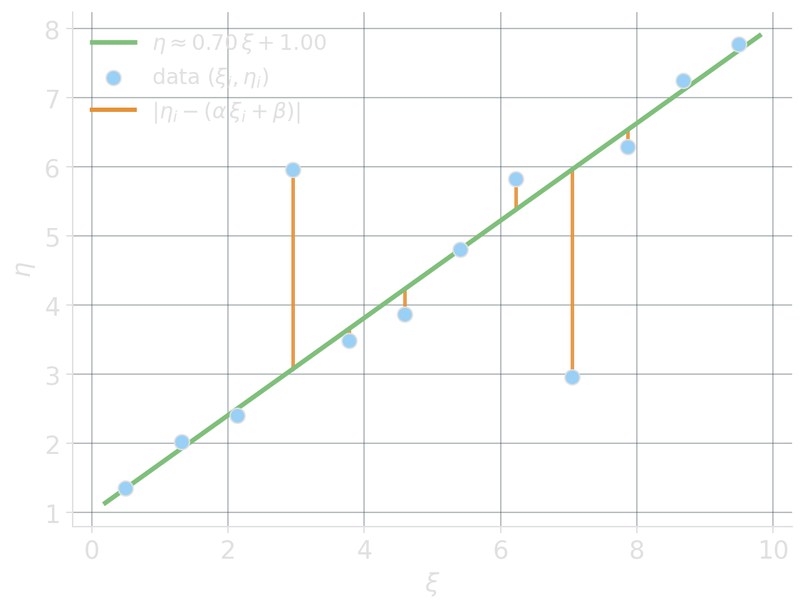
An LP in \(2 + n\) variables: \[ \begin{aligned} \min\quad & \sum_i d_i \\ \text{s.t.}\quad & d_i \ge\ \eta_i - (\alpha\,\xi_i + \beta) && \forall i \\ & d_i \ge\ (\alpha\,\xi_i + \beta) - \eta_i && \forall i \\ & \alpha,\ \beta \in \mathbb{R},\ \ d_i \ge 0. \end{aligned} \]

There are better ways to solve L1 regression than using a general-purpose LP solver.

Learning from Mistakes: Packing Squares with an LP

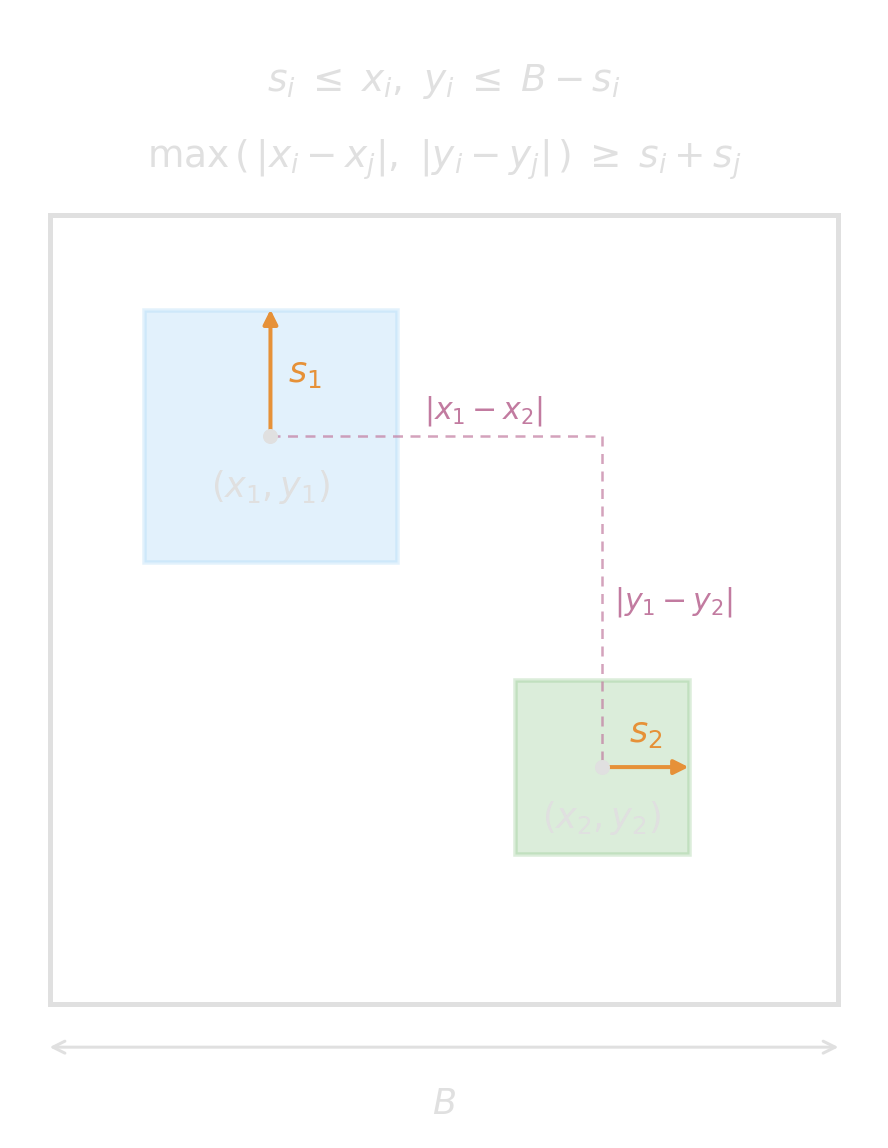
Let us try the trick again: \[ \left. \begin{aligned} d^x_{ij} &\ge x_i - x_j \\ d^x_{ij} &\ge x_j - x_i \end{aligned}\ \right\} \Rightarrow d^x_{ij} \ge \lvert x_i - x_j \rvert \]

Same for the y-axis with \(d^y_{ij}\), and then

\[ \left. \begin{aligned} D_{ij} &\ge d^x_{ij} \\ D_{ij} &\ge d^y_{ij} \end{aligned}\ \right\} \Rightarrow D_{ij} \ge \max(d^x_{ij},\, d^y_{ij}) \]

Will \(D_{ij} \ge s_i + s_j\) guarantee no overlap?

Confucypus says, if your LP solves an NP-hard problem, you probably messed up. Here, we would have needed \(\leq\).

Big-M

The hammer to make nearly anything linear.

What is the Big-M trick?

\[ b = 1 \;\Rightarrow\; a^\top x \le c \quad \Longleftrightarrow \quad a^\top x \le c + M\,(1 - b)\quad \text{ with } M\approx \infty \]

\(b\) constraint meaning
\(1\) \(a^\top x \le c\) active
\(0\) \(a^\top x \le c + M\) relaxed

We can also encode equality \(a^\top x = c\): \[ \begin{aligned} \quad a^\top x \le c + M\,(1 - b) \\ -a^\top x \le -c + M\,(1 - b) \end{aligned} \]


With this, we can easily model, e.g., \(|x| = d\) by introducing two binaries \(b^+\) and \(b^-\):

\[ \left. \begin{aligned} \phantom{-}x &\le \phantom{-}d + M\,(1 - b^+) \\ -x &\le -d + M\,(1 - b^+) \end{aligned} \right\} \text{if } b^+=1 \text{: enforce } d = x \]

\[ \left. \begin{aligned} -x &\le \phantom{-}d + M\,(1 - b^-) \\ \phantom{-}x &\le -d + M\,(1 - b^-) \end{aligned} \right\} \text{if } b^-=1 \text{: enforce } d = -x \]

\[ b^+ + b^- = 1, \quad d \ge 0. \quad \text{(Exactly one branch active, and $d$ non-negative.)} \]

Min and Max

\(d = \min(x, y)\) with binary \(b\):

\[ d \le x, \quad d \le y \]

\[ \left. \begin{aligned} d &\ge x - M\,(1 - b) \\ d &\ge y - M\,b \end{aligned} \right\} \small\text{select which is smaller} \]

\(b\) active result
\(1\) \(d \ge x, d \le x, d \le y\) \(d = x\)
\(0\) \(d \ge y, d \le x, d \le y\) \(d = y\)

\(d = \max(x, y)\) with binary \(b\):

\[ d \ge x, \quad d \ge y \]

\[ \left. \begin{aligned} d &\le x + M\,(1 - b) \\ d &\le y + M\,b \end{aligned} \right\} \small\text{select which is larger} \]

\(b\) active result
\(1\) \(d \le x, d\ge x, d\ge y\) \(d = x\)
\(0\) \(d \le y, d\ge x, d\ge y\) \(d = y\)

For n-ary min or max, introduce one binary per candidate and an exactly-one constraint to select the active branch.

Packing squares as a MIP

\[ \max(|x_i - x_j|, |y_i - y_j|) \ge s_i + s_j \]

can be enforced by \[ \begin{aligned} & x_j - x_i &\ge s_i + s_j - M(1 - b^{R}_{ij}), \\ & x_i - x_j &\ge s_i + s_j - M(1 - b^{L}_{ij}), \\ & y_j - y_i &\ge s_i + s_j - M(1 - b^{A}_{ij}), \\ & y_i - y_j &\ge s_i + s_j - M(1 - b^{B}_{ij}), \end{aligned} \] \[ b^{L}_{ij} + b^{R}_{ij} + b^{A}_{ij} + b^{B}_{ij} = 1. \]

“Need to be separated either from the left, the right, above, or below.”

The Base LP Relaxation doesn’t give us any Information

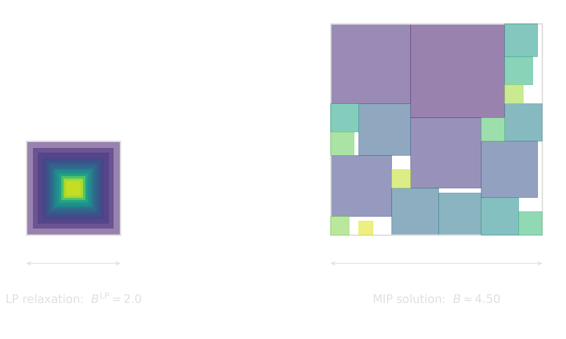
\[ b^{L}_{ij} = b^{R}_{ij} = b^{A}_{ij} = b^{B}_{ij} = 0.25 \]

\[ \begin{aligned} & x_j - x_i \ge s_i + s_j - M(1 - 0.25), \\ & x_i - x_j \ge s_i + s_j - M(1 - 0.25), \\ & y_j - y_i \ge s_i + s_j - M(1 - 0.25), \\ & y_i - y_j \ge s_i + s_j - M(1 - 0.25), \end{aligned} \]

The larger \(M\), the weaker the constraint in the relaxation. In this case, the relaxation is particular weak because even a tight \(M\approx 4\) (why is this tight?) gives too much slack and nearly all constraints are impacted.

But not all is lost!

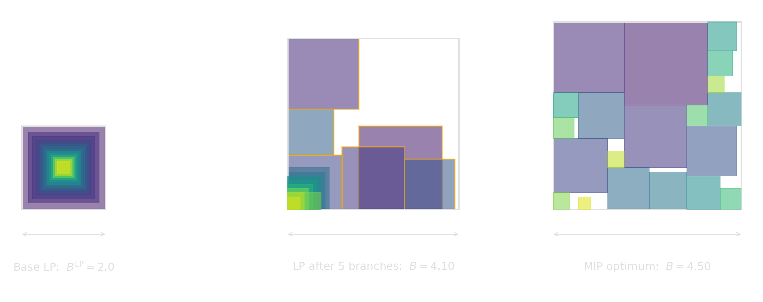
Fixing just five \(b^*_{ij}\) binaries among the largest squares lifts the LP bound from \(2.0\) to \(4.10\), closing most of the gap to the MIP optimum \(B^\star \approx 4.50\). Each branch turns one Big-M slack off and forces a real separation.

Big-M in one slide

  1. Expressiveness. A binary \(b\) and a large \(M\) turn a switch into a linear constraint: \(a^\top x \le c + M(1-b)\).
    • Disjunctions, implications, on/off costs, fixed charges all fit the same template.
  2. The price: not LP-preserving. Fractional \(b\) plus \(M\)-slack collapse the relaxation.
    • Root bound can be near-useless.
    • Branch-and-bound has to rebuild the structure node by node.
  3. Tighten \(M\) when you can. Bounds on the variables shrink \(M\) and the LP gap directly.
    • The formulation stays as weak as the weakest \(M\) you cannot tighten.
  4. Let the solver help. Gurobi (and others) accept indicator constraints \(b = 1 \Rightarrow a^\top x \le c\) directly.
    • Solver picks its own reformulation: inferred \(M\), disjunctive branching, or cuts.
    • No need to commit to a single \(M\) upfront.

Adding Logic

Big-M controlled by boolean logic allows expressing nearly anything.

At-most-one, exactly-one, implication

Counting

\[ \sum_i b_i \le 1 \quad \text{at most one} \]

\[ \sum_i b_i = 1 \quad \text{exactly one} \]

\[ \sum_i b_i \ge 1 \quad \text{at least one} \]

Implication \(b_1 \Rightarrow b_2 \equiv b_1 \;\le\; b_2\).

\(b_1\) \(b_2\) \(b_1 \Rightarrow b_2\) \(b_1 \le b_2\)
\(0\) \(0\)
\(0\) \(1\)
\(1\) \(0\)
\(1\) \(1\)

Negation: \(\;\lnot b \;\equiv\; (1 - b).\)

With at least one and negation, we can already enforce any Boolean function on binaries. However, if we want, e.g., to do \((b_1 \vee b_2) \Rightarrow c^\top x \le d\), we need the AND and OR bindings on the next two slides.

AND-Binding

\[ z = b_1 \land b_2 \quad\Longleftrightarrow\quad z \le b_1, \;\; z \le b_2, \;\; z \ge b_1 + b_2 - 1. \]

\(b_1\) \(b_2\) \(z\) \(b_1 \land b_2\) \(z \le b_1\) \(z \le b_2\) \(z \ge b_1+b_2-1\)
0 0 0 \(= 0\)
0 0 1 \(\neq 0\)
0 1 0 \(= 0\)
0 1 1 \(\neq 0\)
1 0 0 \(= 0\)
1 0 1 \(\neq 0\)
1 1 0 \(\neq 1\)
1 1 1 \(= 1\)

General \(n\)-ary form. \(z = \bigwedge_{i=1}^n b_i \;\Longleftrightarrow\; z \le b_i \;\;\forall i, \;\; z \ge \sum_{i=1}^n b_i - (n-1).\)

OR-Binding

\[ z = b_1 \lor b_2 \quad\Longleftrightarrow\quad z \ge b_1, \;\; z \ge b_2, \;\; z \le b_1 + b_2. \]

\(b_1\) \(b_2\) \(z\) \(b_1 \lor b_2\) \(z \ge b_1\) \(z \ge b_2\) \(z \le b_1+b_2\)
0 0 0 \(= 0\)
0 0 1 \(\neq 0\)
0 1 0 \(\neq 1\)
0 1 1 \(= 1\)
1 0 0 \(\neq 1\)
1 0 1 \(= 1\)
1 1 0 \(\neq 1\)
1 1 1 \(= 1\)

General \(n\)-ary form. \(z = \bigvee_{i=1}^n b_i \;\Longleftrightarrow\; z \ge b_i \;\;\forall i, \;\; z \le \sum_{i=1}^n b_i.\)

Complex Domains

A binary \(b\) activates a continuous \(x\): either off (zero) or live (in a range).

Semi-Continuous Variables

\(x\) is either \(0\) or lies in \([L, U]\) with \(0 < L \le U\):

\[ x \in \{0\} \cup [L, U] \qquad\Longleftrightarrow\qquad L\, b \le x \le U\, b, \quad b \in \{0, 1\}. \]

\(b\) \(L\, b \le x\) \(x \le U\, b\) \(x\)
\(0\) \(0 \le x\) \(x \le 0\) \(= 0\)
\(1\) \(L \le x\) \(x \le U\) \(\in [L, U]\)

The same \(b\) doubles as a fixed-charge switch: add \(c\, b\) to the objective and you pay \(c\) whenever \(x \neq 0\).

Segmented Domains

\(x\) lies in one of several disjoint intervals:

\[ x \in [L_1, U_1] \cup [L_2, U_2] \cup [L_3, U_3]. \]

Reusing one shared \(x\) with three semi-continuous blocks pins \(x\) to zero — every off-block forces \(x = 0\) simultaneously.

Split \(x\) into one continuous part per interval; an exactly-one selector picks the live part:

\[ x = x_1 + x_2 + x_3, \quad L_k\, b_k \le x_k \le U_k\, b_k, \quad b_1 + b_2 + b_3 = 1. \]

\((b_1, b_2, b_3)\) \(x_1\) \(x_2\) \(x_3\) \(x = \sum_k x_k\)
\((1, 0, 0)\) \(\in [L_1, U_1]\) \(= 0\) \(= 0\) \(\in [L_1, U_1]\)
\((0, 1, 0)\) \(= 0\) \(\in [L_2, U_2]\) \(= 0\) \(\in [L_2, U_2]\)
\((0, 0, 1)\) \(= 0\) \(= 0\) \(\in [L_3, U_3]\) \(\in [L_3, U_3]\)

Piecewise-linear approximation

When the function itself is nonlinear, approximate with line segments and commit.

How do we model this?
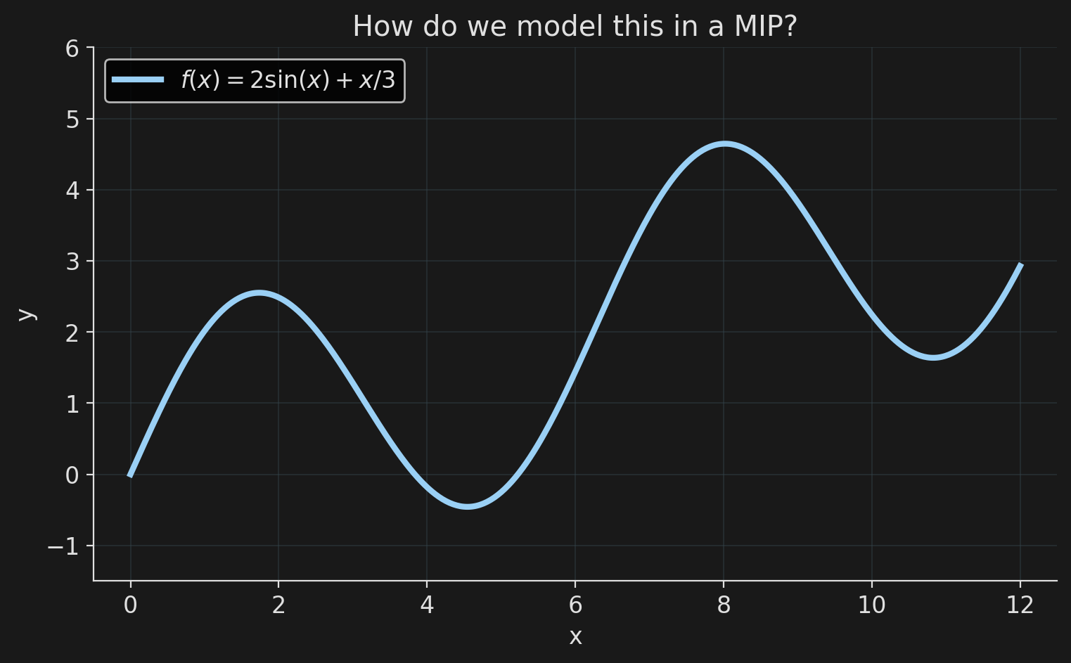
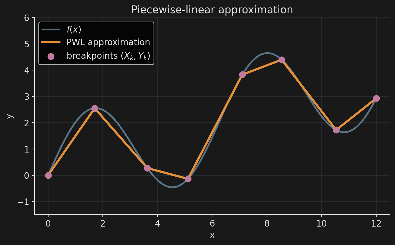
Encoding the PWLA

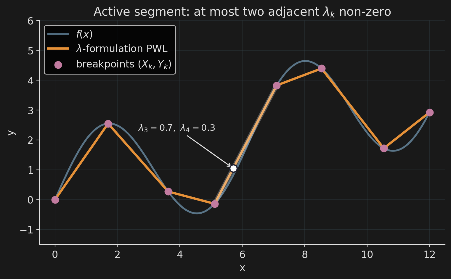
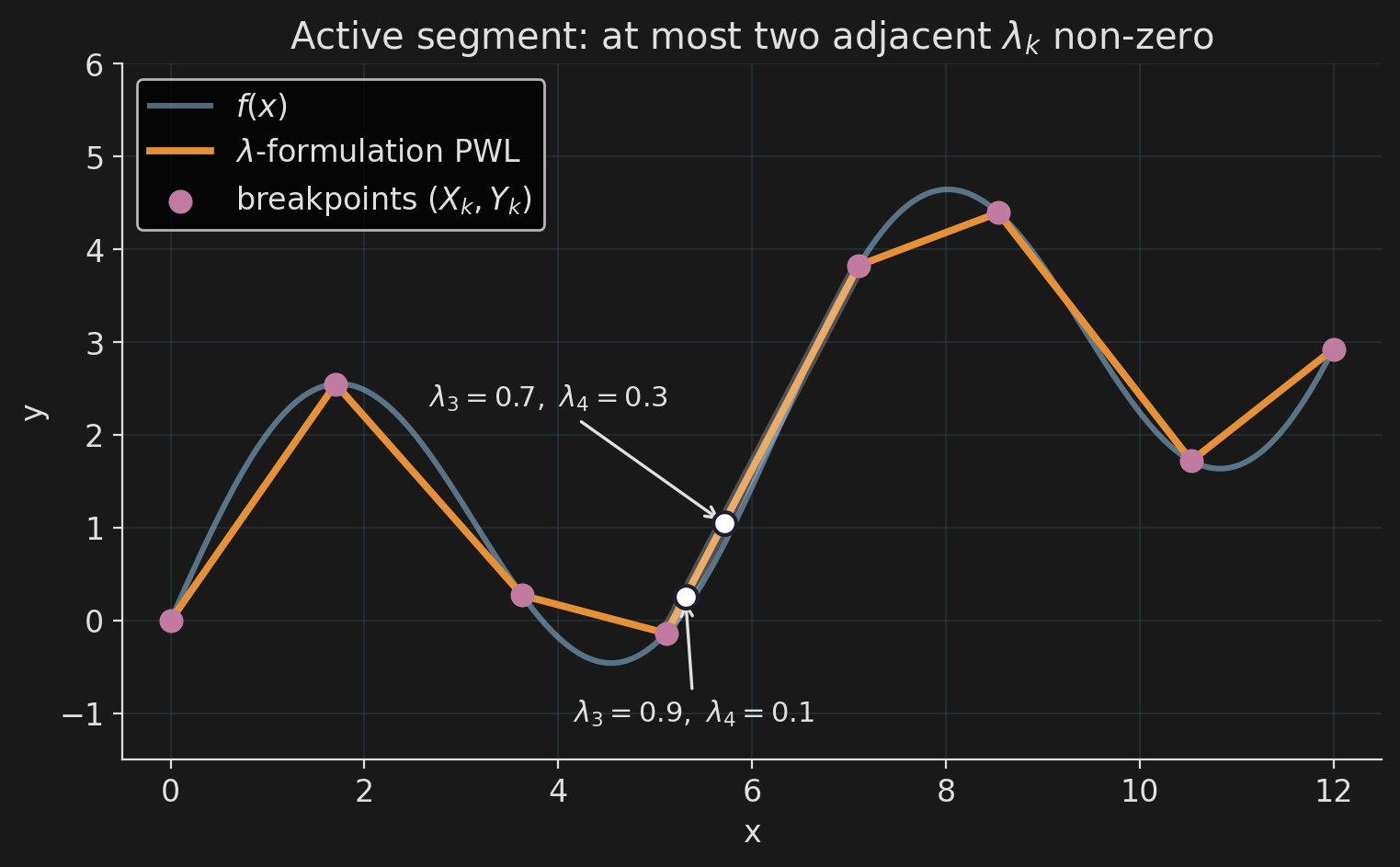
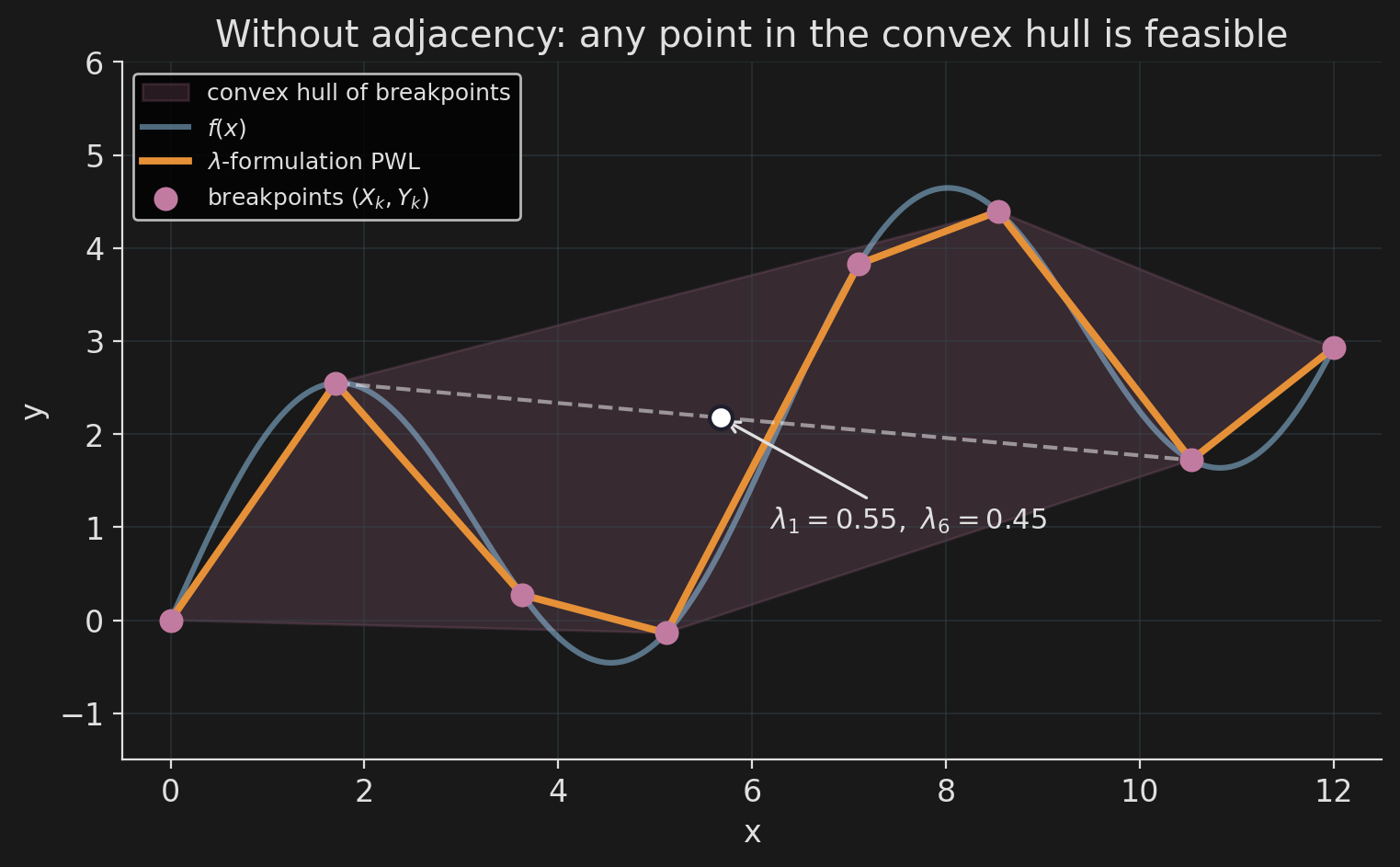
Breakpoints \((X_k, Y_k)\) are data. Each \(x\) is a convex combination of the \(X_k\); \(y\) uses the same weights:

\[ x = \sum_k \lambda_k\, X_k, \qquad y = \sum_k \lambda_k\, Y_k, \qquad \sum_k \lambda_k = 1, \;\; \lambda_k \ge 0. \]

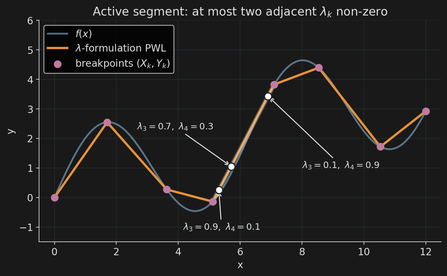
Adjacency. Only two consecutive \(\lambda_k\) may be non-zero. One activation binary \(b_k\) per segment:

\[ \lambda_0 \le b_0, \quad \lambda_K \le b_{K-1}, \]

\[ \lambda_k \le b_{k-1} + b_k, \quad \sum_k b_k = 1. \]

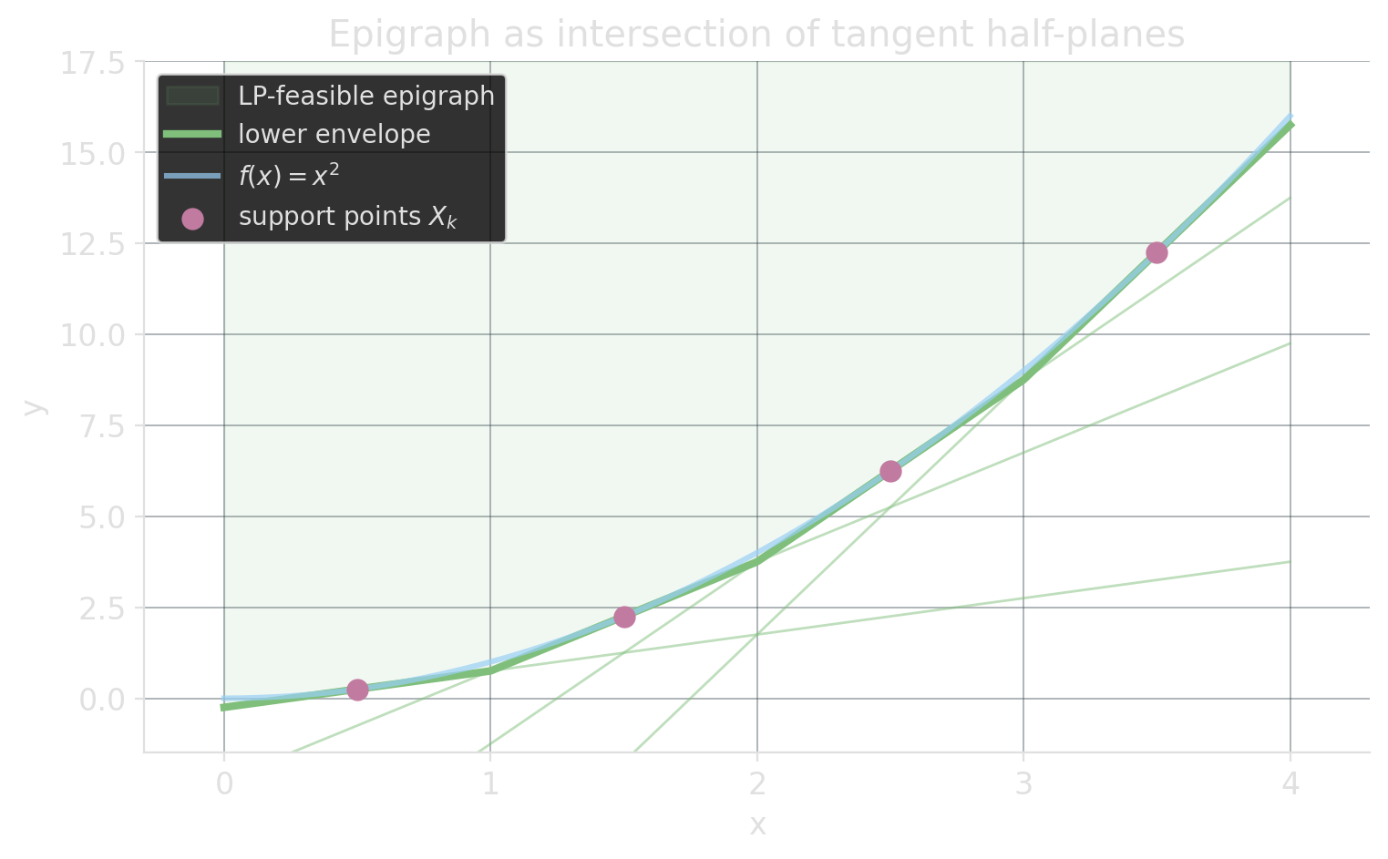
Convex functions: no binaries needed

For convex \(f\), the epigraph \(\{(x, y) : y \ge f(x)\}\) is itself convex. Tangent half-planes from below give an LP-only encoding:

\[ y \;\ge\; f'(X_k)\, (x - X_k) + f(X_k) \qquad \text{for each chosen support } X_k. \]

The LP picks the binding tangent automatically: objective pressure pulls \(y\) down to the envelope. No binaries.

Only enforces \(y \ge f(x)\). Equality \(y = f(x)\) still needs segment-selection binaries.

Non-linear solvers do PWLA in secret

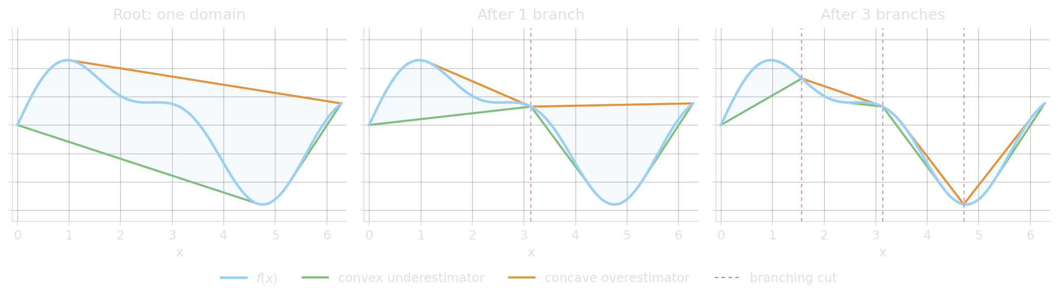
Some non-linear solvers approximate the function with convex/concave envelopes, branch on the variable’s domain, and refine the envelopes on every child node. Linear relaxations all the way down: an LP solver underneath, solving a non-linear problem.

Strong vs weak formulations

Two correct models can present very different LPs to branch-and-bound.

Facility location: open some sites, serve all customers

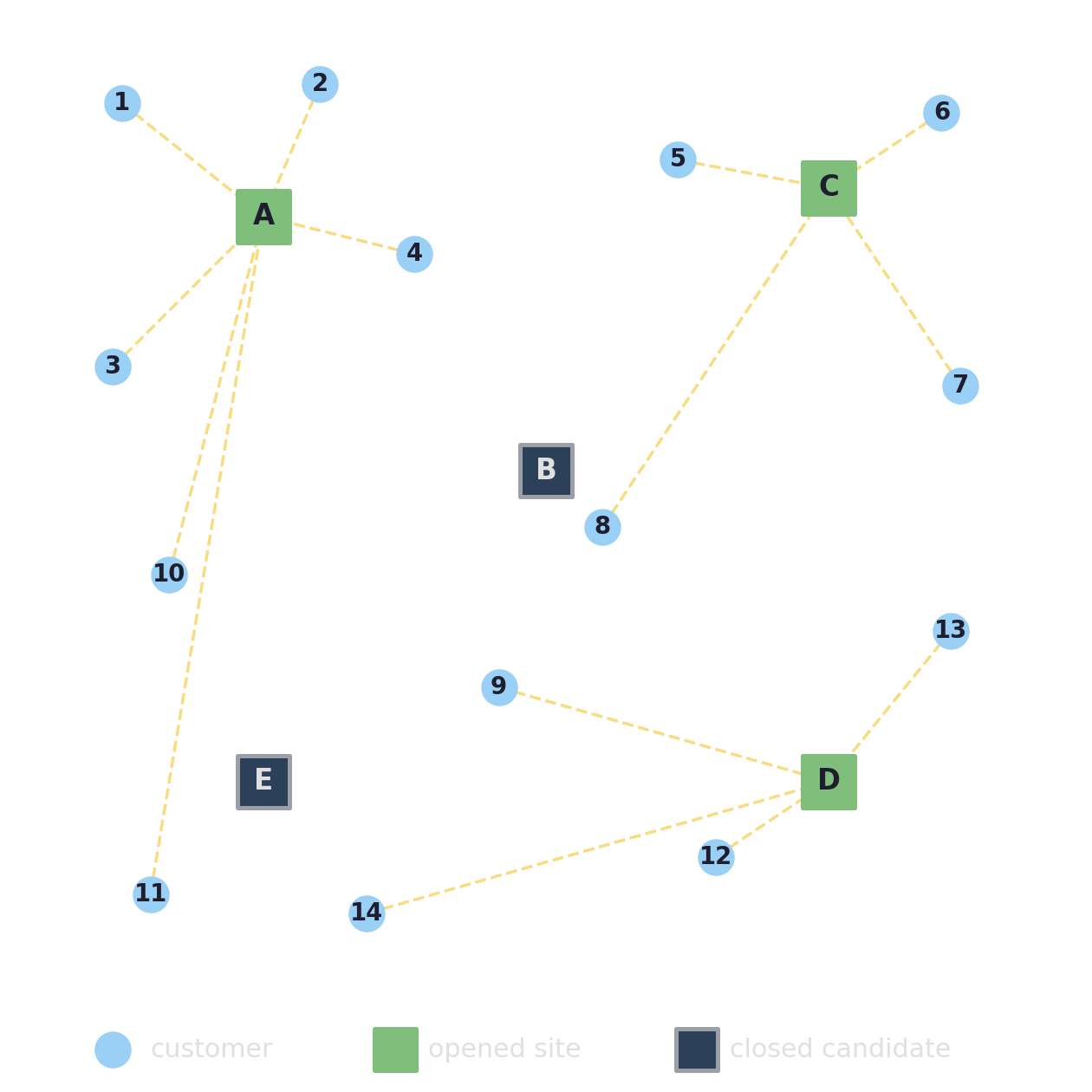
Customers need to be served from depots. Each candidate site \(j\) has a fixed opening cost \(f_j\); each pair carries a shipping cost \(c_{ij}\).

Pick which sites to open and how to assign every customer to an open site so that the total cost (opening plus shipping) is as small as possible.

TSP subtour elimination: pick your poison

MTZ (directed).

\[ \begin{aligned} \min \;\; & \sum_{i \ne j} c_{ij}\, x_{ij} \\ \text{s.t.} \;\; & \textstyle\sum_{j \ne i} x_{ij} = 1 \quad \forall i \\ & \textstyle\sum_{i \ne j} x_{ij} = 1 \quad \forall j \\ & \color{#e69138}{\color{#3d85c6}{u_j} \;\ge\; \color{#3d85c6}{u_i} + 1 - n\,(1 - x_{ij})} \\ & \color{#e69138}{\qquad \forall i \ne j,\ i, j \ge 1} \\ & x_{ij} + x_{ji} \le 1 \quad \forall i < j \\ & x_{ij} \in \{0,1\},\ \color{#3d85c6}{u_0 = 0},\ \color{#3d85c6}{u_i \in [1, n{-}1]} \end{aligned} \]

DFJ (undirected).

\[ \begin{aligned} \min \;\; & \sum_{e \in E} c_e\, x_e \\ \text{s.t.} \;\; & \textstyle\sum_{e \in \delta(i)} x_e = 2 \quad \forall i \in V \\ & \color{#e69138}{\textstyle\sum_{e \in \delta(S)} x_e \ge 2} \\ & \color{#e69138}{\qquad \forall\, \emptyset \subsetneq S \subsetneq V} \\ & x_e \in \{0,1\} \end{aligned} \]

Big-M (\(n\)) → weak LP relaxation.

\(2^n - 2\) constraints → tight but unwritable.

The separation theorem

Grötschel–Lovász–Schrijver (1981). An LP can be optimized in polynomial time iff its separation problem can be solved in polynomial time.

Separation: given \(\hat x\), return a violated constraint or certify there is none.

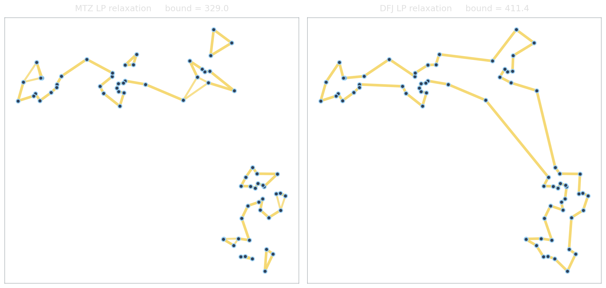
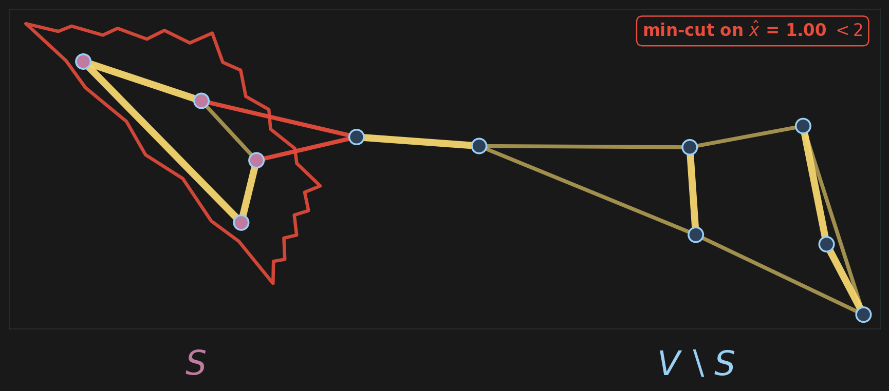
For DFJ, separation is min-cut on the graph weighted by \(\hat x\): cut value \(< 2\) yields a violated subtour inequality.

Confucypus says: under LP duality, variables are constraints and constraints are variables. The dual of separation is column generation.

The complexity of an LP is not defined by its naive size.

The LP relaxations, side by side

Some formulations are already integral

For some problem classes, every vertex of the LP polytope is integer. Simplex returns an integer optimum directly: no branching, no cuts. The “relaxation” is the algorithm.

Classical examples.

  • Bipartite matching, assignment
  • Min-cost flow, max-flow / min-cut, transportation
  • Shortest path (as LP)
  • Interval scheduling, point covering by intervals
  • General-graph matching (Edmonds’ odd-set inequalities)

The usual sufficient condition is total unimodularity of \(A\) (Hoffman–Kruskal, 1956): then \(B^{-1}b\) is integer for any integer \(b\), so every basic solution is integer.

Brittle. A single fixed-charge, budget, or precedence constraint usually destroys integrality and pushes the model back onto the strong-vs-weak spectrum.

See you next time