Real-World Optimization Problems
Algorithm Engineering — T04
JSSP, Rostering, VRP
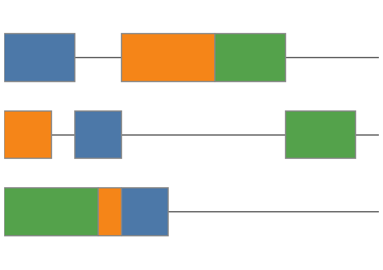
Shop scheduling
Tasks → machines, over time.
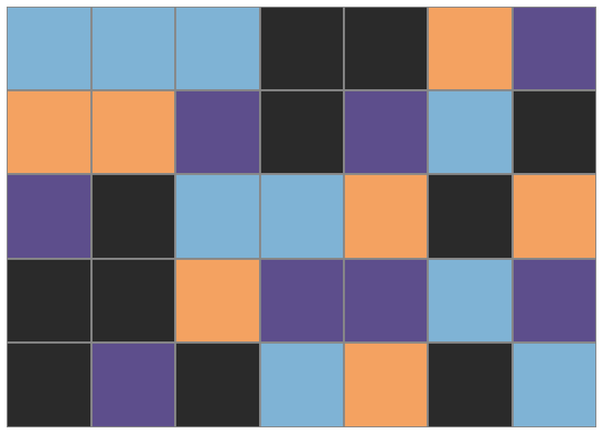
Employee rostering
People → shifts, over a horizon.
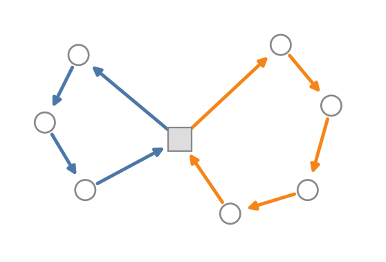
Vehicle routing
Stops → vehicles, in space and time.
The classical Job Shop

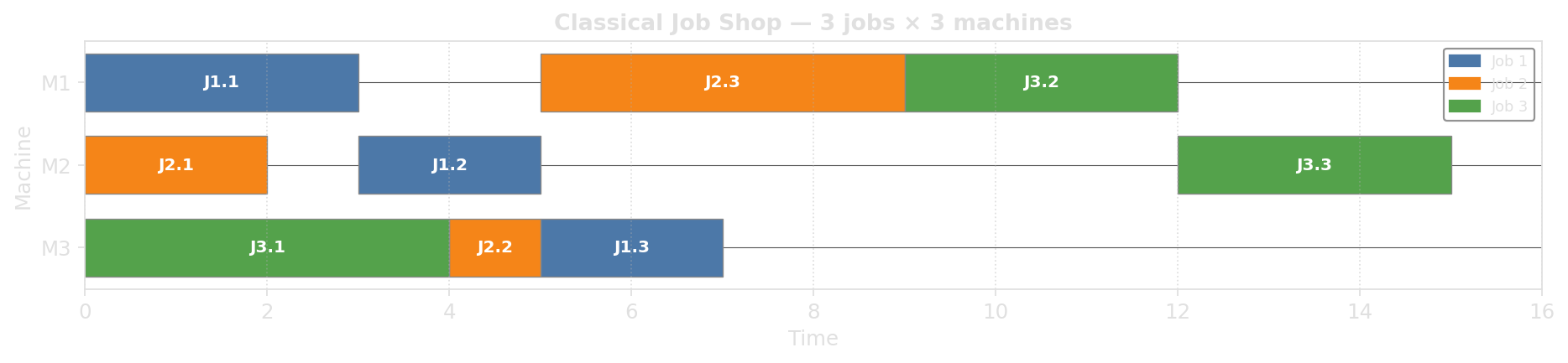
Variant: Flexible Job Shop
Each task can run on one of several eligible machines, with possibly different durations.
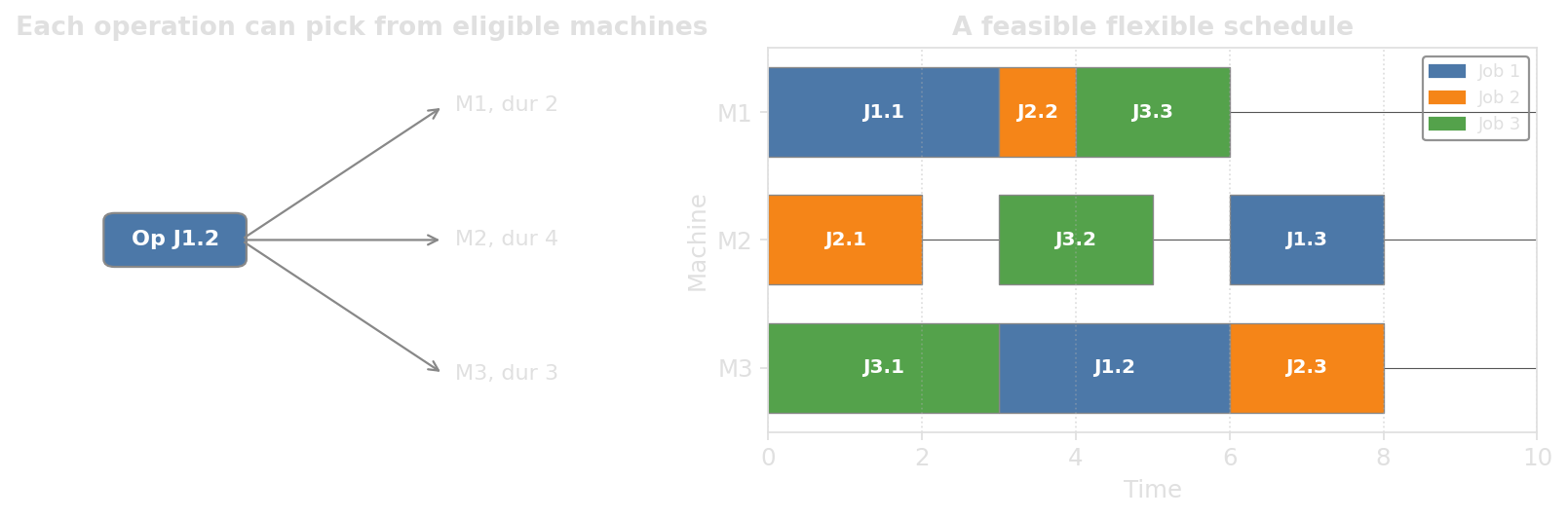
We now decide which machine and when. The search space multiplies; balancing load gets easier; the model gets harder.
Variant: Flow shop
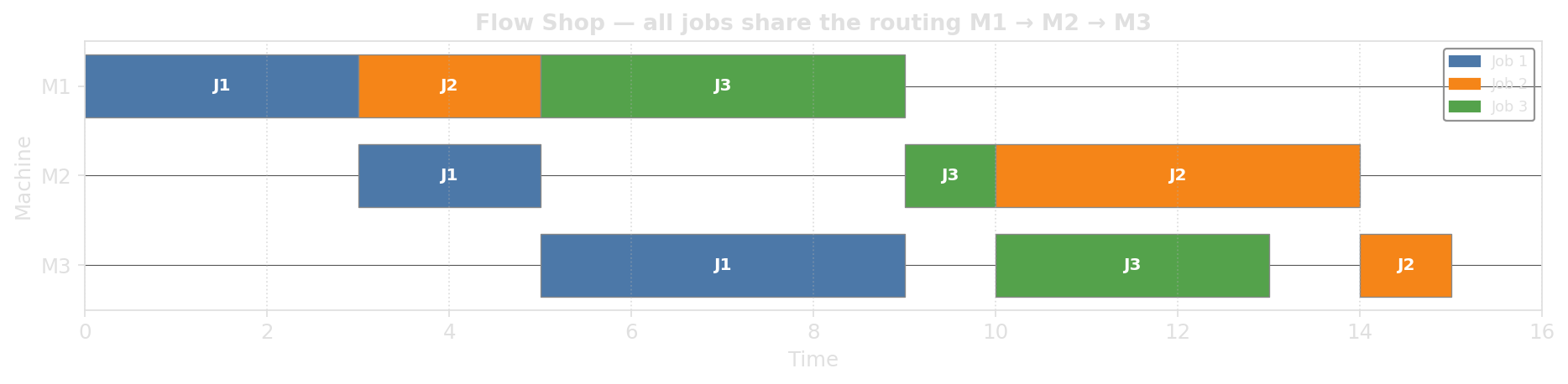
Every job visits the machines in the same order, but jobs may overtake each other on later stages.
The classic assembly-line layout: stamp, then weld, then paint, then assemble. Routings collapse to a single shared sequence, so the only decision left is the order in which jobs enter the line.
Variant: Permutation flow shop
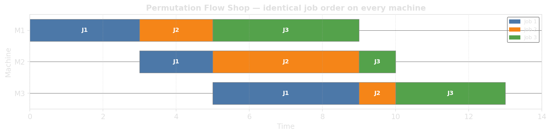
Flow shop plus no overtaking: every machine sees the jobs in the same order.
What a literal conveyor belt enforces: once you are ahead at station one, you stay ahead everywhere. Far smaller search space (pick one permutation), but still NP-hard from three stages on.
Variant: Hybrid flow shop
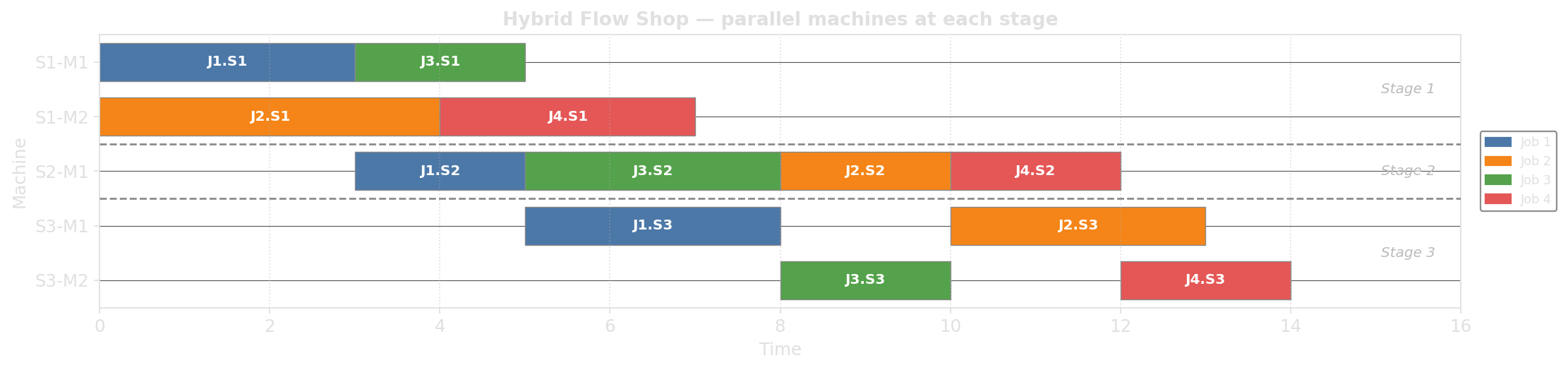
Flow shop, but each stage has a pool of parallel machines.
A common topology in volume manufacturing: stamping, welding, painting, final assembly each run on several near-identical stations. Within a stage, the solver assigns jobs across machines; between stages, the flow constraint still applies.
Variant: Open shop
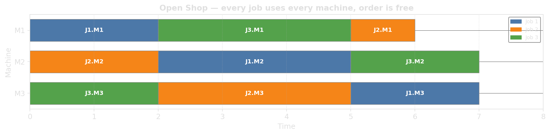
Each job visits each machine once, but the order is free.
Maintenance checklists, independent lab analyses on one sample, parallel test suites on shared hardware: anywhere the steps can run in any order. The extra freedom packs tighter schedules at the cost of a much larger decision space.
Variant: Project scheduling (RCPSP)
Change: tasks no longer block a whole machine; they consume a quantity of a resource.
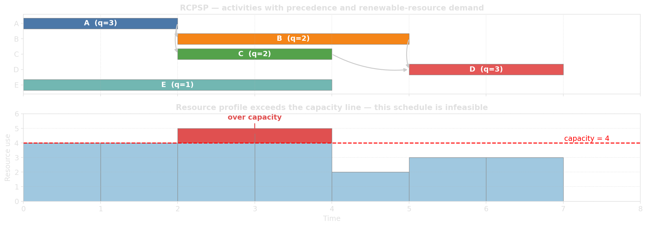
The schedule above violates capacity: at \(t \in [2,4)\) demand reaches 5 but only 4 is available (red block).
A valid schedule keeps total demand under capacity at every moment, e.g. by delaying an activity until the resource frees up.
Variant: Multi-mode activities
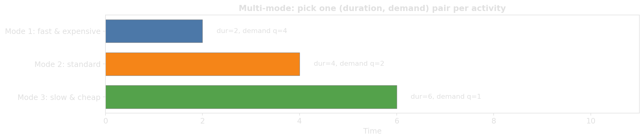
Each task has several modes with different duration / resource trade-offs.
Rent more workers and finish faster, or work with the small crew and take longer. Picking the mode is now part of the optimization.
Variant: Consumable resources
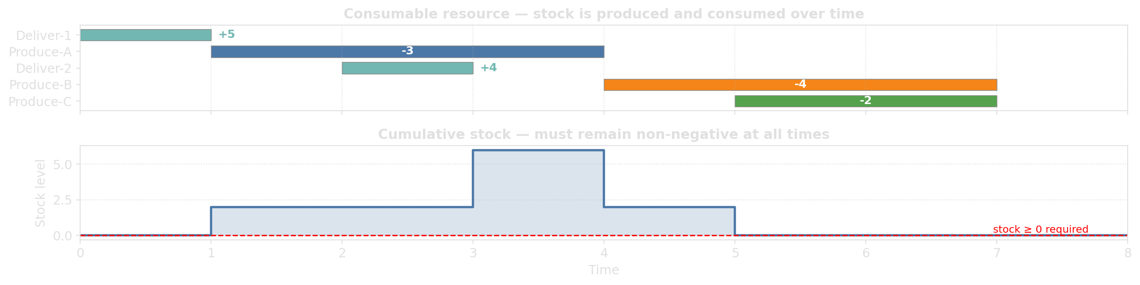
Resources deplete until something tops them up; stock must stay non-negative at every moment.
Renewable resources come back (workers go home, fuel up, return). Consumables don’t: raw material, screws, money, fuel. This couples producing tasks to consuming tasks in a way the renewable model cannot capture.
Constraint: Sequence-dependent setups
Between two tasks on the same machine, a setup is needed whose length depends on both the previous and the next task.
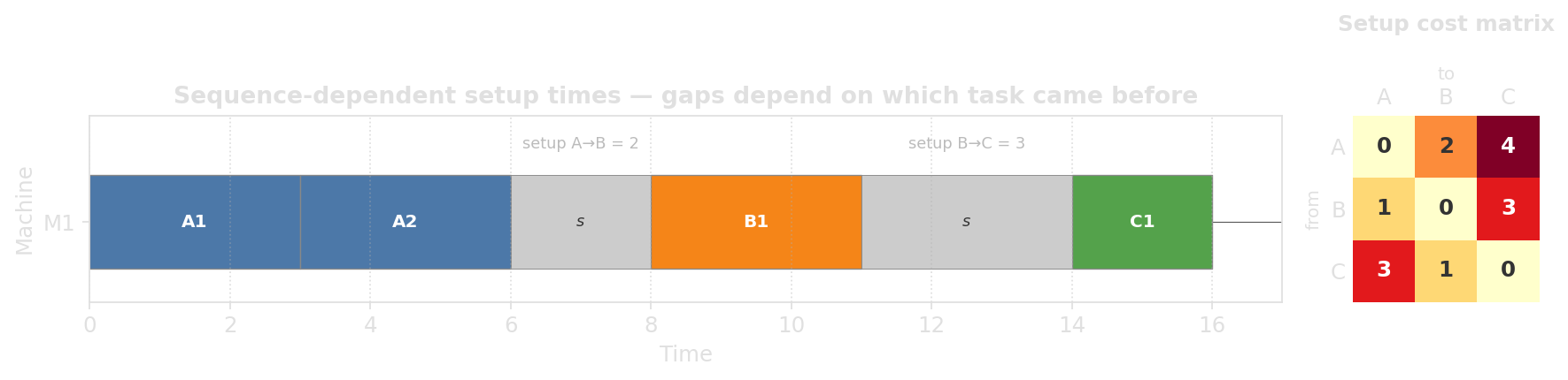
Order on each machine now affects cost; the problem inherits TSP-like structure per machine.
Constraint: No-wait and blocking
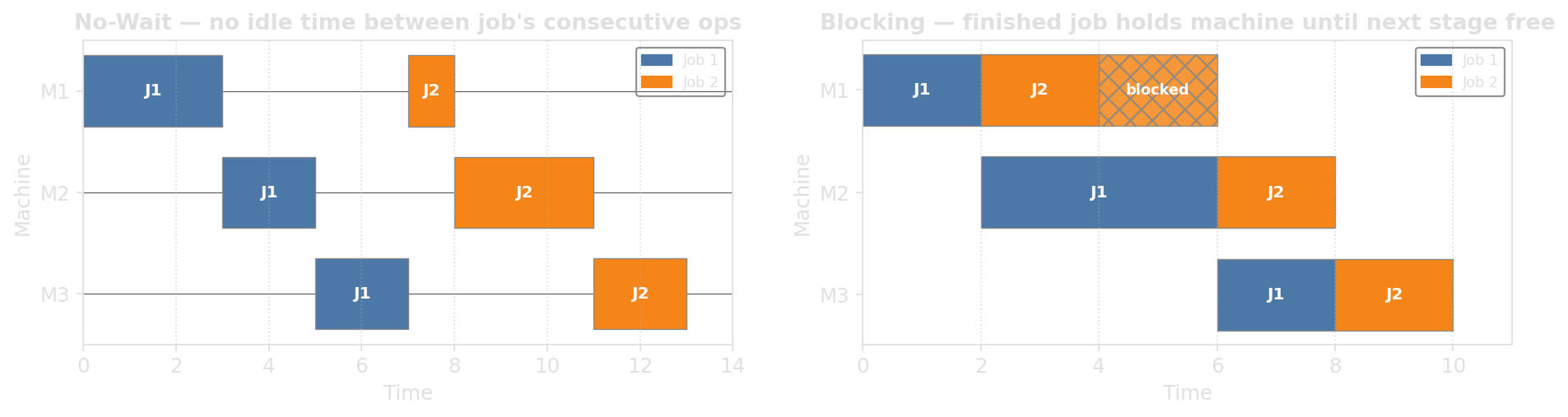
Two flavors of “no buffer between stages”:
No-wait
Once a job starts, no idle time between tasks. Steel rolling, food, chemistry.
Blocking
No buffer between stages: a finished job occupies its machine until the next stage is free.
Constraint: Resource breaks
Resources are not available 24/7: lunch breaks, weekends, maintenance windows.
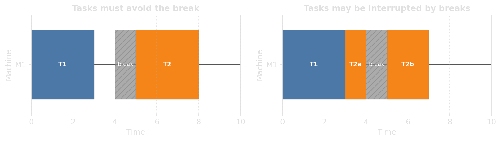
Shift patterns are a frequent production-floor request, in both the “must avoid” and “interruptible” flavors.
Constraint: Optional tasks
Not every task has to be executed. We pick which tasks to schedule.
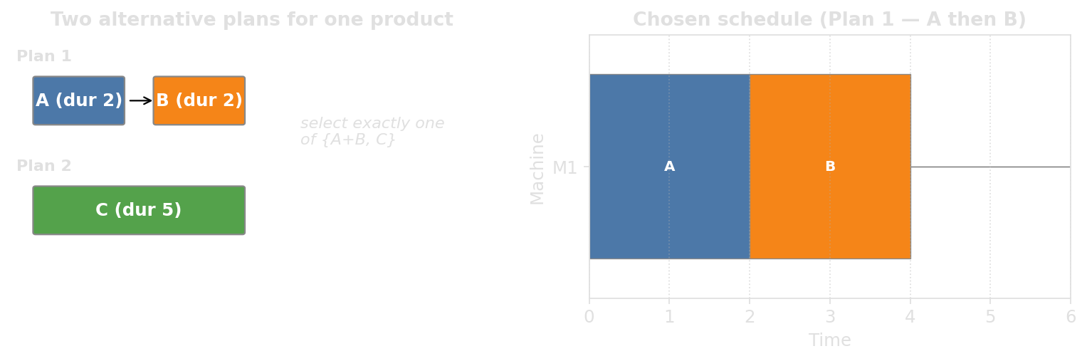
Use cases: alternative process plans, scheduling with rejections, “all-or-none” job structures.
Constraint: Time windows
Each job has time-window information.
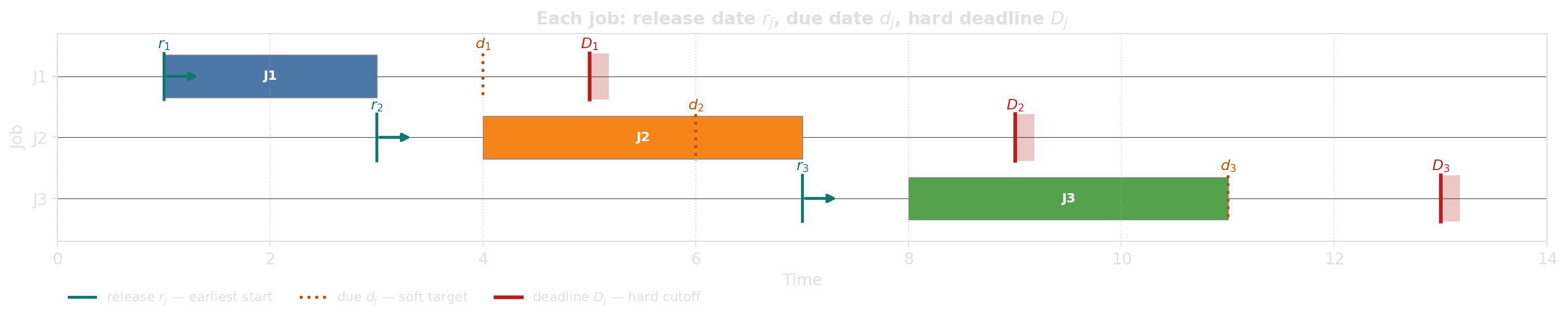
- Release date \(r_j\): earliest start (raw material arrives)
- Due date \(d_j\): soft target; missing it costs but is allowed
- Deadline \(D_j\): hard cutoff; missing it is infeasible
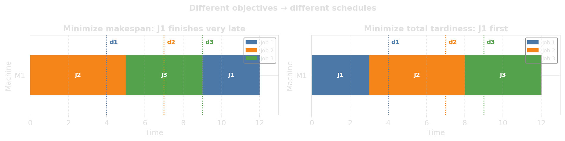
Objective changes the schedule
| Objective | Formula | When it matters |
|---|---|---|
| Makespan \(C_{\max}\) | finish time of last job | Throughput, batch production |
| Total tardiness \(\sum T_j\) | \(\sum \max(0, C_j - d_j)\) | Service-level penalties |
| Tardy jobs \(\sum U_j\) | how many miss their due date | SLA breach count |
| Max tardiness \(T_{\max}\) | worst late job | Fairness, contractual caps |
| Total flow time \(\sum C_j\) | sum of completion times | Average customer wait |
| Setup time | sum of setup gaps | Energy, wear |
The core problem
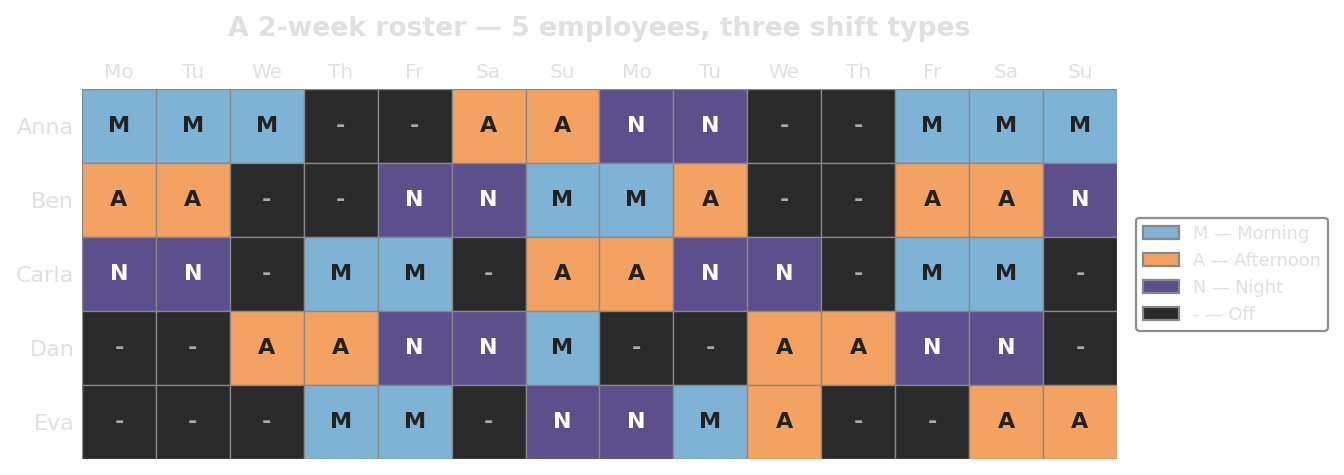
Inputs: planning horizon split into shifts; coverage demand per shift; pool of employees with contracts, skills, availability, preferences.
Output: a roster matrix: for every (employee, day) cell, the assigned shift (or off).
Hard vs soft constraints
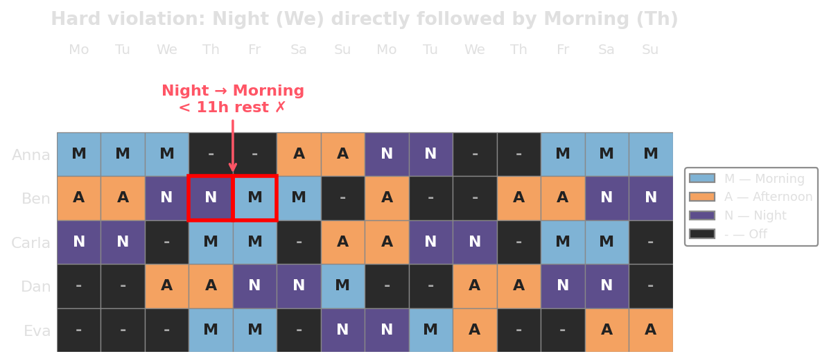
Hard: law, safety, contract. Violation means infeasible. Soft: preferences, fairness, nice-to-haves. Violation is allowed but penalized.
Modern solvers use a multi-level score \((\text{hard}, \text{medium}, \text{soft})\) compared lexicographically: hard must be zero before soft is even looked at.
Coverage requirements
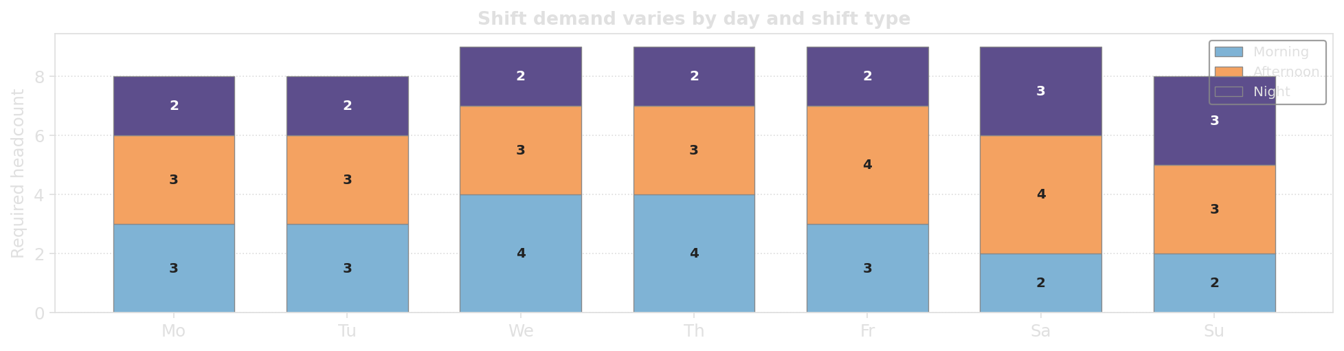
- Skill-mix coverage: “three staff, at least one with pediatric certification”
- Min/max coverage: lower and upper bounds per shift
- Time-of-day demand: continuous staffing curves discretized into micro-shifts
Skills and availability
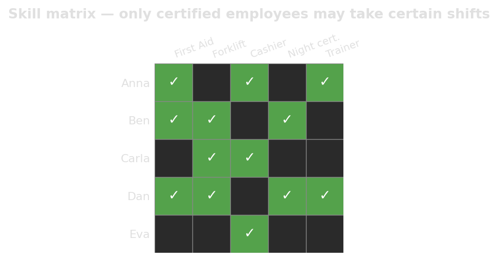
Skills Who can do what.
Availability Who is available when.
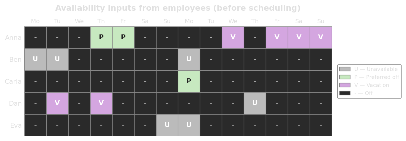
“When Beth has next Friday off for a wedding party, she should not be assigned to a shift on that Friday.”
Rest periods
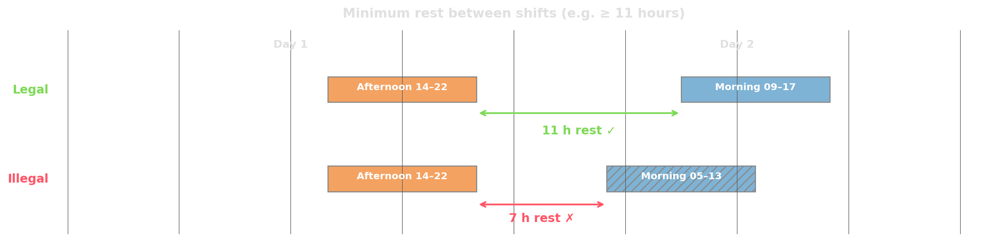
- Minutes between shifts: explicit minimum gap
- Consecutive minutes off in rolling window: long rest within any 7-day window
- Shift start-time differences: limit day-to-day variation (circadian rhythm)
- Forbidden shift pairings: even with 14h rest, “night → morning” is bad practice
Weekends
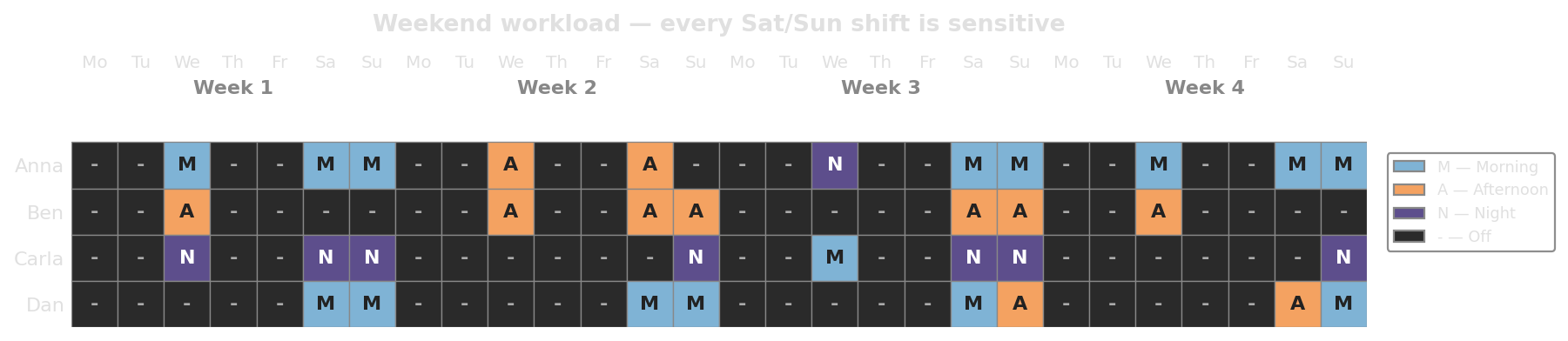
- Max weekends worked per 4-week window (e.g. ≤ 2 of 4).
- Consecutive weekends off (everyone gets a free weekend).
- Whole-weekend coupling (work Saturday → also work Sunday).
- Weekend equity across staff.
Fairness and workload balance
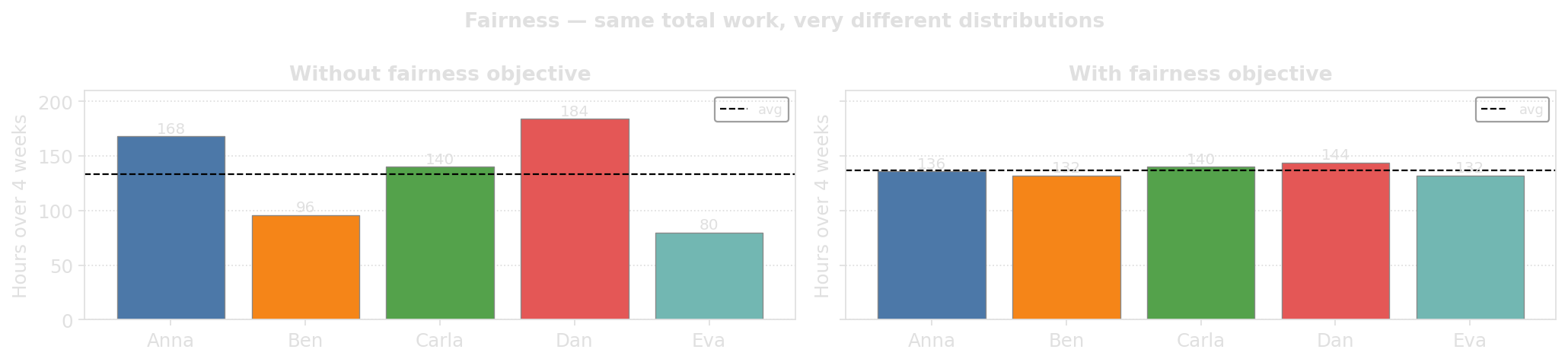
A “technically feasible” roster that always lands the night shifts on the same person is not feasible in any meaningful sense. They quit.
Contracts
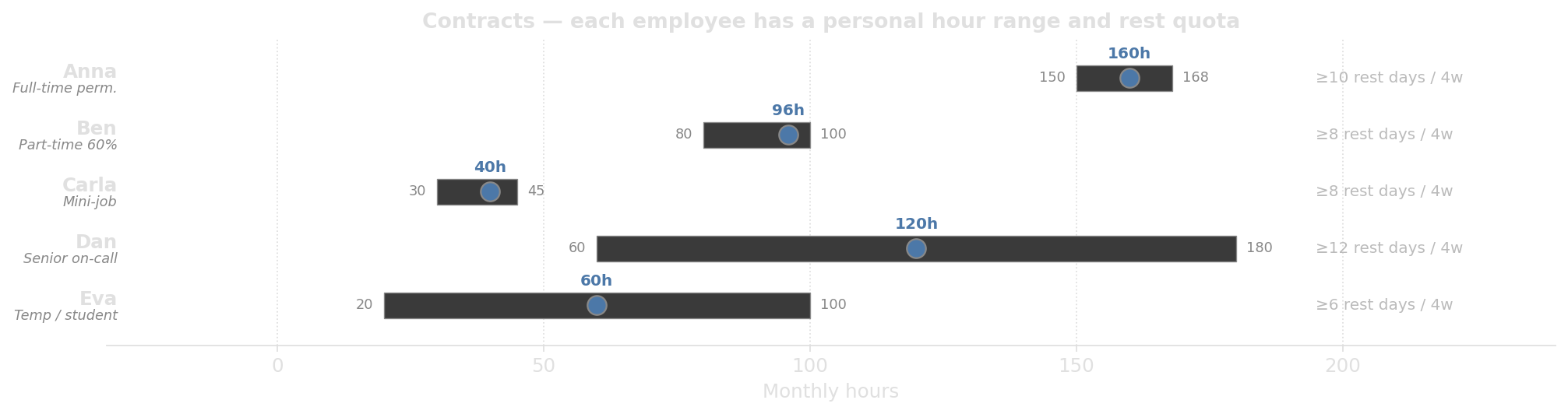
A contract typically specifies:
- A monthly hour range \([\min, \max]\) and a planned target within it.
- Maximum consecutive days worked, minimum rest days per period.
- A subset of eligible shift types (e.g. “no nights for trainees”).
- An employee priority that decides whose preferences carry more weight.
Preferences
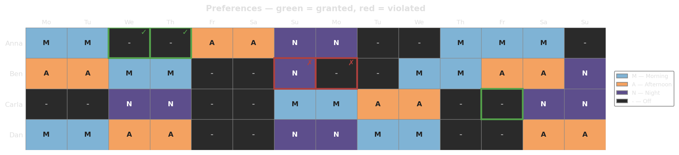
Some staff prefer night shifts; others would rather keep specific evenings free for childcare, training, or a second job.
Granting non-conflicting preferences costs the employer nothing and improves retention.
Shift patterns and rotations
Many organizations use rotating schedules instead of re-solving from scratch each cycle.
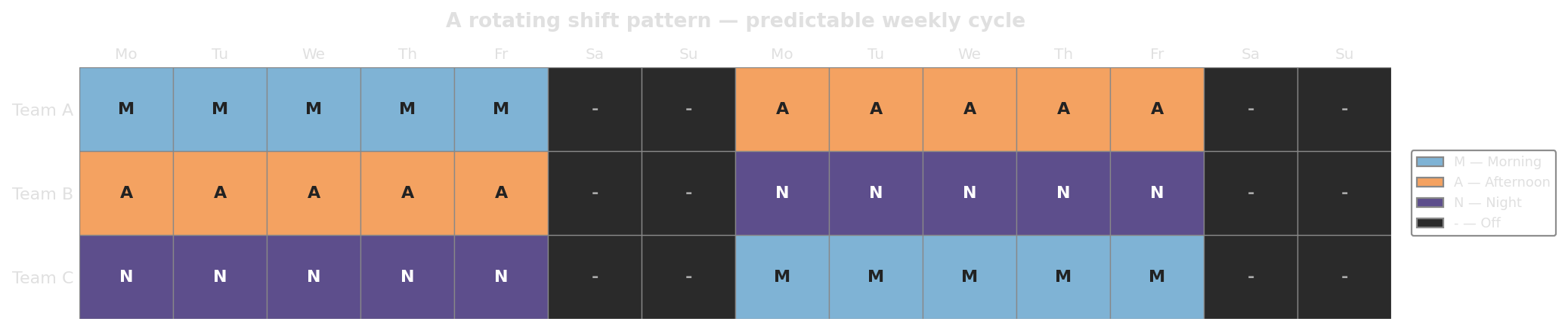
Rotations trade flexibility for predictability. Most real systems use a rotating base pattern with ad-hoc overrides.
Pairing and location constraints
Some assignments come in groups, not individually.
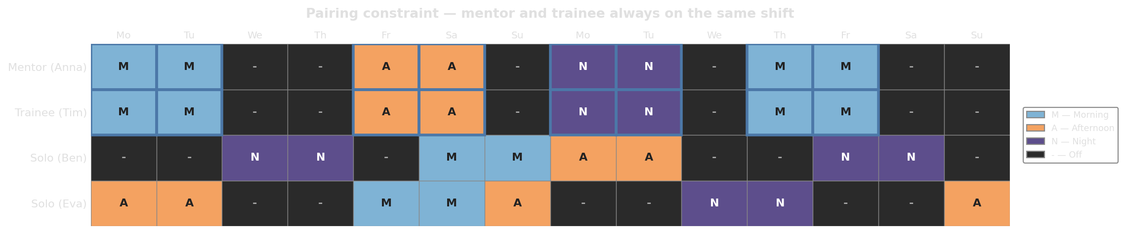
| Type | Example | Hard? |
|---|---|---|
| Required pair | New hire must always be paired with mentor | ✓ |
| Preferred pair | Two employees who carpool together | ✗ |
| Prohibited pair | Couple whose HR policy forbids same-shift work | ✓ |
| Unpreferred pair | Siblings alternating eldercare | ✗ |
The core problem
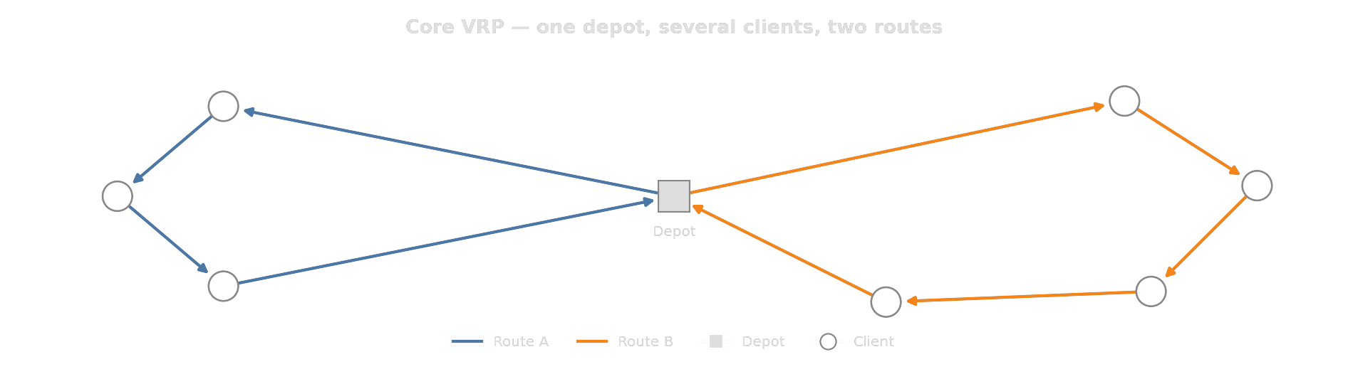
One depot, a set of clients, a fleet of vehicles.
Visit every client exactly once, every route starts and ends at the depot, minimize total cost.
Variant: Capacity (CVRP)
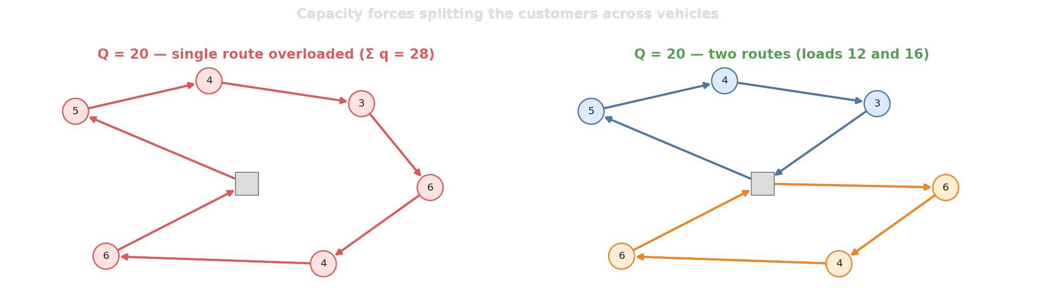
Without it, one vehicle would always do everything; capacity is what determines the fleet size.
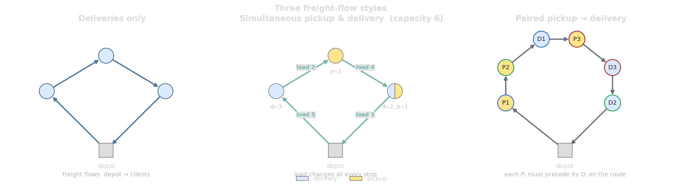
Variant: Pickups and deliveries
Variant: Time windows (VRPTW)
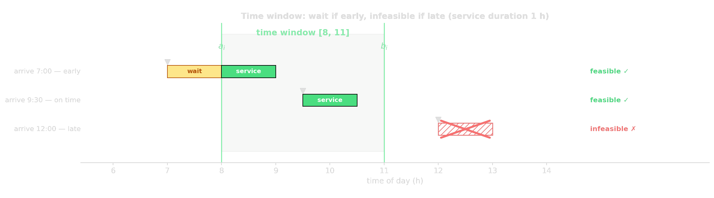
Clients are not always available all day.
Time windows couple the sequence of visits to the clock. Two clients close in space may be impossible to serve on one route because their windows conflict.
Variant: Driver shifts
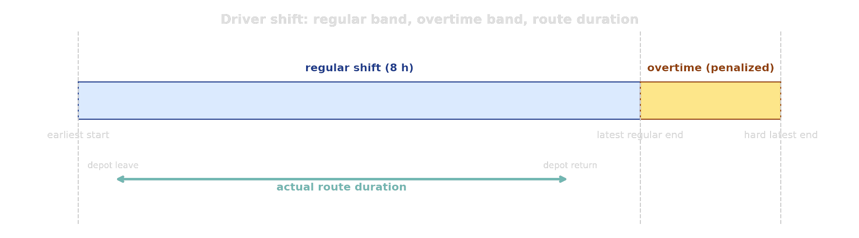
Earliest start, latest end, overtime band: usually a soft limit.
Variant: Hours-of-service breaks
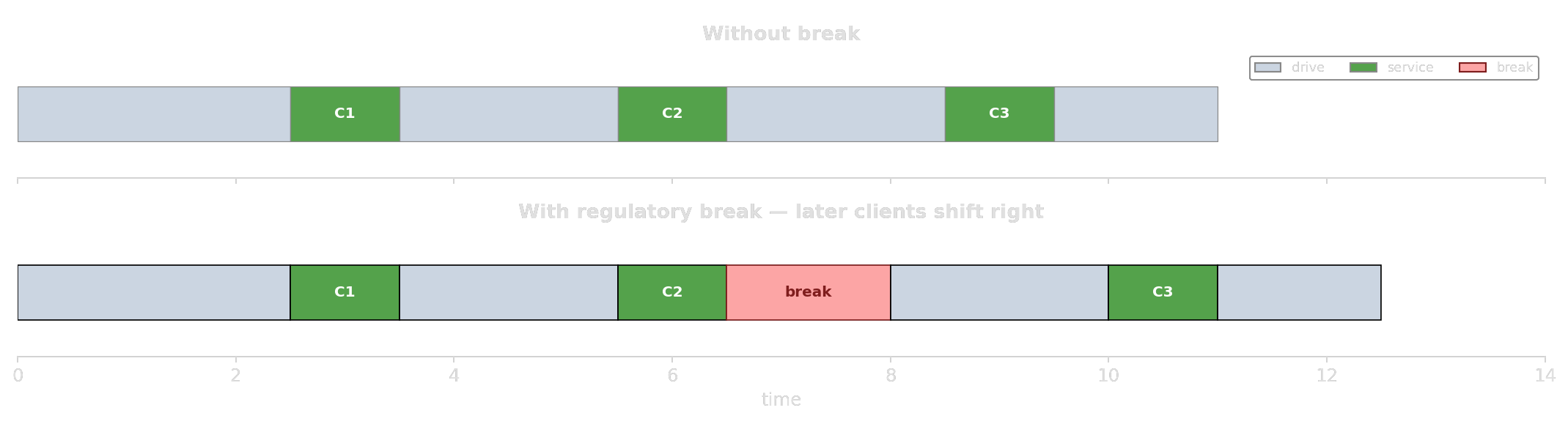
EU/US law: 45-min break after 4.5h of driving.
The break is not at a fixed time. Where it lands in the schedule, and at which location, is itself a decision, and it shifts every later arrival downstream.
Variant: Multiple depots
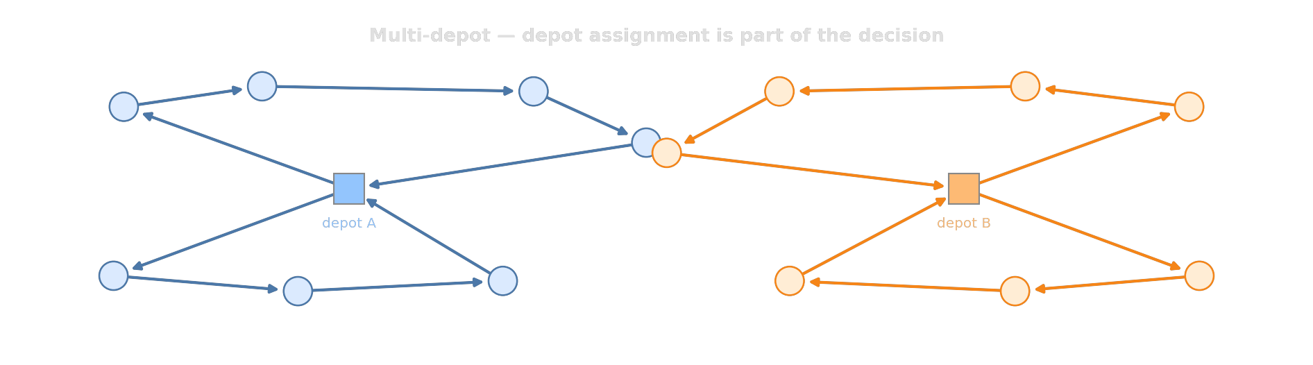
Which depot serves which client is part of the problem, not an input.
Variant: Heterogeneous fleet (routing profiles)
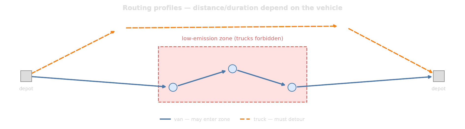
Distance and duration matrices depend on the vehicle type.
Variant: Reloading and multi-trip
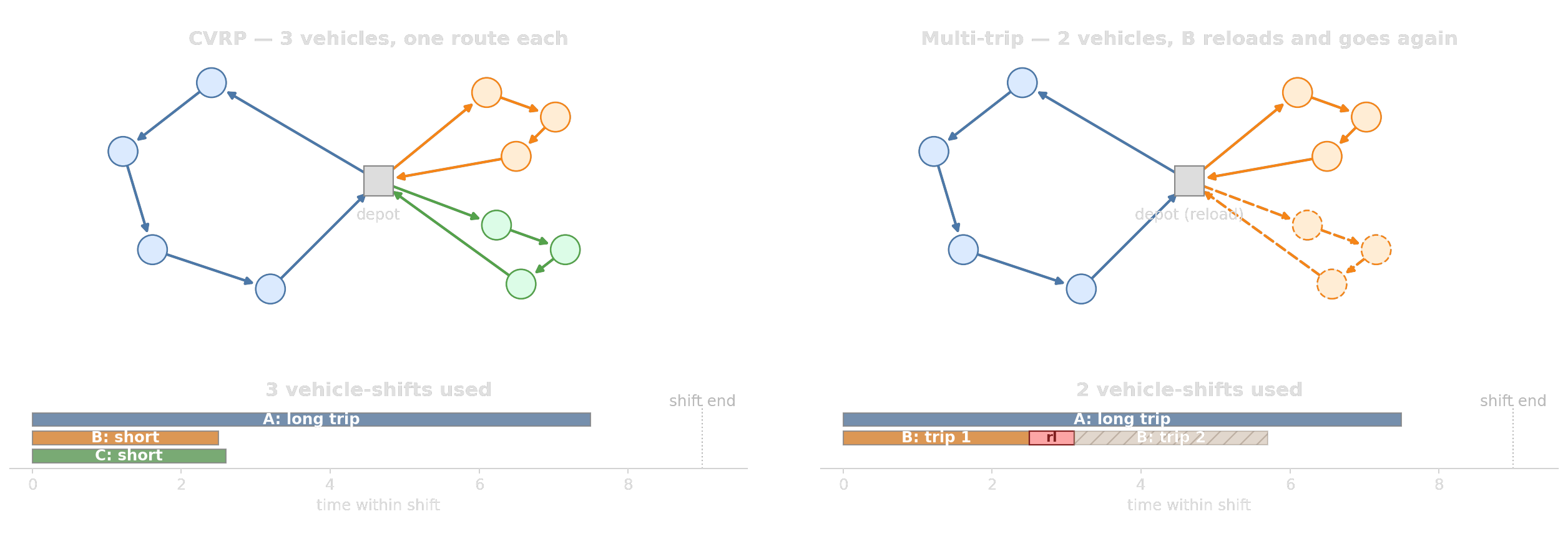
- Capacity still binds per trip; that is why we reload.
- Across the whole shift, the bottleneck is driving hours, not vehicle size.
Variant: Prize collection (optional clients)
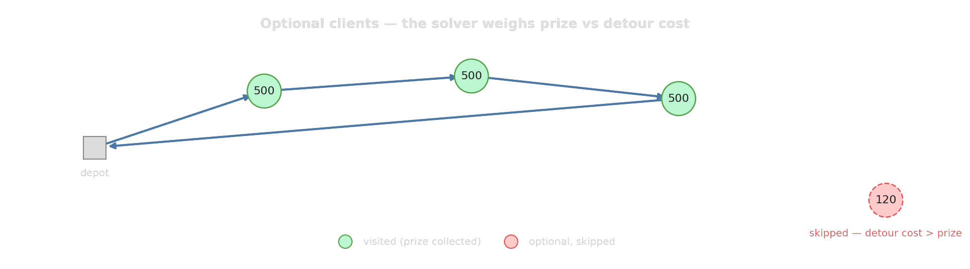
Not every job has to be done today. Each client carries a prize \(\pi_i\):
\[\min \;\text{routing cost} - \sum_{i \text{ visited}} \pi_i\]
Variant: Mutually exclusive client groups
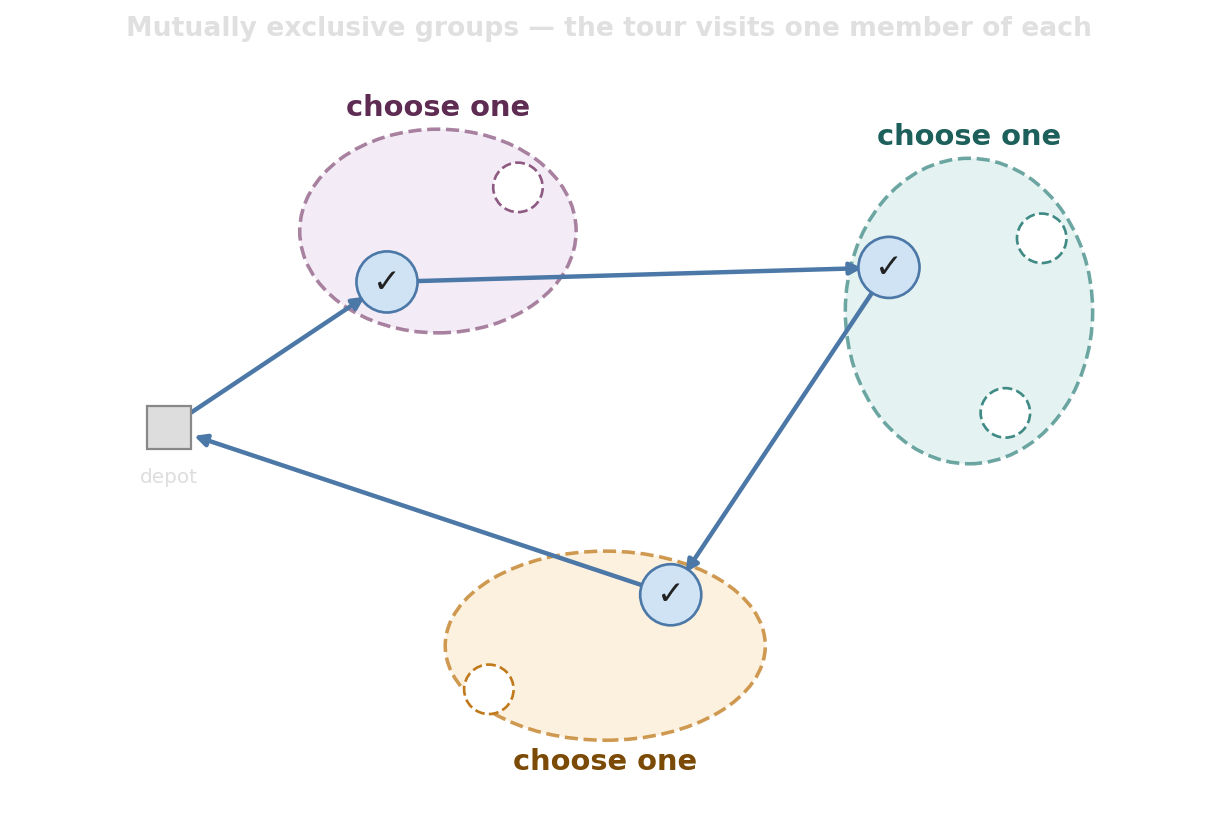
“Exactly one of”:
- Drop the package at the front desk or at the parcel locker.
- Service the customer in the morning slot or the evening slot.
- Visit one of three branches of the same chain.
The tour visits exactly one member of each group; the solver picks which.
JSSP, Rostering, VRP
Shop scheduling
- Flexible job shop
- Flow / hybrid / open shop
- Project scheduling (RCPSP)
- Multi-mode, consumables
- Sequence-dependent setups
- No-wait / blocking
- Resource breaks, time windows
PyJobShop · CP-SAT
Rostering
- Coverage requirements
- Skills & availability
- Rest periods, weekends
- Contracts, working hours
- Fairness & balance
- Preferences
- Patterns, pairing, replanning
Timefold · SolverForge
Vehicle routing
- Capacity (CVRP)
- Pickups & deliveries
- Time windows (VRPTW)
- Driver shifts, HOS breaks
- Multiple depots, mixed fleet
- Reloading / multi-trip
- Prize collection, client groups
PyVRP · OR-Tools